Bridging the yield gap

GRDC project code: CSA00042

Authors

Zvi Hochman, Ecosystem Sciences/Sustainable Agriculture Flagship, CSIRO, Dutton Park, Australia.

David Gobbett, Ecosystem Sciences/Sustainable Agriculture Flagship, CSIRO, Glen Osmond, Australia.

Heidi Horan, Ecosystem Sciences/Sustainable Agriculture Flagship, CSIRO, Dutton Park, Australia.

Di Prestwidge, Ecosystem Sciences/Sustainable Agriculture Flagship, CSIRO, Dutton Park, Australia.

Javier Navarro Garcia, Ecosystem Sciences/Sustainable Agriculture Flagship, CSIRO, Dutton Park, Australia^.

Introduction

Growth in global grain production has all but stalled (Grassini et al., 2013) yet the FAO estimate that  global food security will require world grain production to increase by at least 60% between 2010 and 2050 (Alexandratos and Bruinsma, 2012). This is both a huge challenge for the world’s agronomists and an exciting opportunity for Australia’s grains industry. One promising pathway for increasing grain production is by closing the gap between yields currently achieved on farms and those that can be achieved by using the best adapted crop varieties and best crop and land management practices for a given environment (van Ittersum et al., 2013).

When discussing yield potential and possible new management practices that may be helpful to raise farm production it is important to define the terms used to benchmark production: 

• Ya = Actual yield: yields achieved in commercial fields. Reflecting farmers’ natural endowment, access to technology, and their skill and exposure to real market economics (Evans and Fischer, 1999 as adapted by Hochman et al., 2009)
• Yw = Water-limited yield: simulated yield for the same conditions, climatic and crop management, as for Yatt, except for N supply which is non-limiting (Hochman et al., 2012).  Yw as defined here applies to current best practice. New technology can re-define Yw by increasing the production frontier
• Yg = Yield gap for rain-fed crops:  the difference between Yw and Ya
• Y_% = Relative yield: calculated as 100 x Ya/Yw (Lobell et al., 2009)
• Exploitable yield gap: the difference between Y_% = 80% and Ya. Based on observations that farmers’ yields plateau at 80% of Yw, probably due to diminishing returns to investment and aversion to risk (Lobell et al., 2009; van Ittersum et al., 2013).

Before you can bridge the yield gap you need to know big it is! While farmers could sustainably aim for about 80% of their water limited yields, they first need to know what their target is and how close there are to achieving it. Advisers are already aware of the gap between their best and worst farmers but do they know to what extent this is determined by their environment or their Yw?

This talk is about a web based tool that will allow farmers and their advisers to benchmark their own wheat yields against the water limited wheat yields and the average wheat yields being achieved by others in their statistical local area (SLA).

Methods

A number of steps are required to derive maps of actual yields (Ya), water limited yields (Yw), yield gaps (Yg) and relative yields (Y_%):

1. We obtained a land use map showing areas most likely to have produced winter cereal crops in the 2005 season at a spatial resolution of 1.1 km. This map was generated from ABARE–BRS (2010) dataset. It is based on remotely sensed NDVI data and census information to spatially disaggregate land use within area constraints provided by the agricultural census. A more detailed explanation of the procedure can be found in Bryan et al. (2009). We focused our efforts on all SLAs in Australia that grew a minimum of 5000 ha of wheat. 
2. We determined Ya for each SLA. Farmers are surveyed annually by the Australian Bureau of Agricultural and Resource Economics and Sciences (ABARES) through its Australian Agricultural and Grazing Industries Survey (AAGIS). The annual data for wheat are aggregated up from individual farms to SLAs to 11 regions in three ago-climatic zones. The 11 regions in the Australian wheat-sheep zone are viewed by ABARES as the smallest unit for which their annual survey is designed to produce reliable wheat crop estimates (ABS, 2009). These data are available through the Agsurf website (http://abare.gov.au/ame/agsurf/agsurf.asp). The less frequently sampled Agricultural Census data provide reliable crop estimates at the SLA level. We found that where data existed at both regional and SLA level (17 years of data) there were very strong correlations between regional yield and SLA yields that allowed for reliable prediction of individual SLA yields from regional yields. This allowed us to estimate Ya for 259 SLAs in Australia for all years from 1996 to 2010. A fifteen year period was chosen as it is sufficiently long to represent climate variability but short enough to represent current technology and best practice.
3. We determined Yw by using APSIM simulation of a “continues wheat” crop from 1996 to 2010 for up to three dominant soil types within a 17 km of each of Silo’s met stations (patch point data) within the wheat land use map. A total of 11660 simulations were run to provide data for mapping Yw. The results of the soil types for each met station were weighted by the relative distributions of the soil type in the proximity of the met station. Soil data was derived from APSoil and ASRIS maps. Local kriging was used to smooth out the individual points and determine annual Yw values for each SLA.  
4. We calculated Yg (=Yw-Ya) and Y% (=100 x Ya/Yw) for each SLA and each year and mapped the results.

Results and discussion

The focus in this paper is on results in GRDC’s northern region.  The annual Ya data were mapped into figure 1. These maps illustrate the spatial variability of yields with contrasting results often observed between neighbouring SLAs. This is most dramatically illustrated for 2004 where a blue zone (yields > 2.4 t/ha) borders against a red zone (yields < 1.4 t/ha). Equally the maps illustrate annual climate variability where generally good years like 1996, 1999 and 2010 contrast with years like 2000, 2002, 2006 and 2007.

The data layer for calculating Yw can be summarised by Figure 2 which overlays a map of the SLA boundaries with the winter cereal land use data layer (blue dots, each representing 1.1sq km) and meteorological data stations (diamond shapes) coloured to represent the most dominant soil type in their buffer zone.  While the meteorological data are not uniformly distributed throughout the wheat growing areas, we are most fortunate in Australia to have such comprehensive meteorological and soil data at our disposal.

The annual Yw calculations were mapped into figure 3. As with Figure 1, these maps illustrate the spatial variability of water limited yields with contrasting results often observed between neighbouring SLAs. This is most dramatically illustrated for 2003 where a blue zone (yields > 4.5 t/ha) borders against a red zone (yields < 2.6 t/ha). Similarly, the maps illustrate annual climate variability where generally good years like 1996 1999 and 2010 contrast with years like 2002, 2006 and 2007. It is important to note that the scale of yields used in Figure 3 (from less than 2.6 to greater than 4.5) is higher than that used for Figure 1 (from less than 1.4 to greater than 2.4). This difference indicates the yield gap.

The annual yield gap is mapped in Figure 4. As with Ya and Yw, Yg varies in time and space. Significantly, low yielding years like 2002 tend to have small yield gaps while high yielding years like 2010 have larger yield gaps. There is a strong correlation (r²= 0.72) between Yw and Yg (Figure 5) indicating that across all locations and seasons, the higher the yield potential the higher the yield gap. Maps of annual relative yields still show variations in space and seasons (Figure 6). The predominance of Y_% values less than 43% in 1998 reflects the extreme wet winter experienced in that La Niña year. Widespread waterlogging and crop disease issues associated with a wet winter were the likely causes of the low Y% in 1998. In most years values greater than 63% appear sporadically in some SLAs.    

Average annual values of Ya, Yw, Yg and Y_% (figure 7) per SLA show that some SLAs have larger yield gaps than others. This spatial difference holds true even when the yield gap is expressed as relative yields.  For the 48 SLAs in the northern region Ya = 1.67 t/ha; Yw = 3.58 t/ha; Yg = 1.91 t/ha and Y_% = 46.6%. Compared with the national figures actual yields are lower than in the southern region and similar to the western region. However the northern region has the highest Yw value and thus the largest absolute yield gap and smallest relative yield (Table 1).

Figure 1. Actual wheat grain yields in Australia’s northern grain zone (aggregated at SLA level)

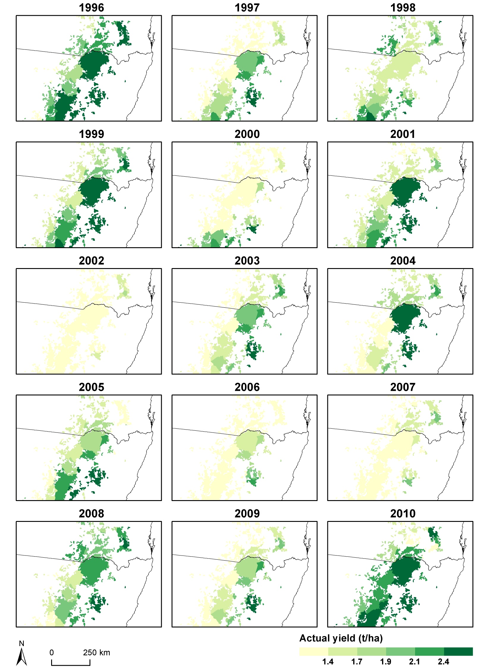
Figure 1 text description:

• In 1996, there was a yield in the central region of approximately 2.5t/ha. The northern region showed a yield of predominantly 2.3t/ha with up to approximately 2.5t/ha. Lower yields of approximately 1.5t/ha were also found. The southern region showed a yields ranging approximately 1.7t/ha to 2.4t/ha. the south western region show a the lowest yield of approximately 1.4t/ha.
• In 1997, the northern region showed a yield of approximately 1.4t/ha with the north east showing a slightly higher yield of approximately 1.7t/ha. The central region showed a yield of approximately 2.0t/ha. The southern region showed a yield ranging from approximately 1.7t/ha to 2.4t/ha with the south east reaching a yield of approximately 2.5t/ha.
• In 1998, the central region showed a yield of approximately 1.6t/ha. The northern region also showed a yield of approximately 1.6t/ha with the north east and north west showing up to approximately 2.3t/ha. The southern region showed a yield ranging from approximately 1.7t/ha to 2.4t/ha in the furthest southern region.
• In 1999, the central region showed a yield of approximately 2.5t/ha. The northern region showed a yield mainly ranging from 1.7t/ha to 2.1t/ha and reaching approximately 2.5t/ha in the north east. The southern region yield ranged from approximately 1.7t/ha to 2.4t/ha in the south east.
• In 2000, the central and norther region showed a yield of approximately 1.4t/ha. The southern region showed a yield of approximately 1.9t/ha with the south east showing up to 2.4t/ha.
• In 2001, the central region showed a yield of approximately 2.5t/ha. The northern region showed a yield ranging from approximately 1.4t/ha to 2.0t/ha. The southern region showed a yield ranging from approximately 1.7t/ha to 2.4t/ha in the south east.
• In 2002, all regions showed a yield of approximately 1.3t/h. The yield increased to approximately 1.6t/ha in some areas in the north east and south east.
• In 2003, the central region showed a yield of approximately 2.1t/ha. The northern region showed a yield of approximately 1.4t/ha in the north west to approximately 2.1t/ha in the north east. The southern region showed a yield of approximately 1.4t/ha in the south west to approximately 2.5t/ha in the south east.
• In 2004, the central region showed a yield of approximately 2.5t/ha. The northern region showed a yield of approximately 1.7t/ha and up to 2.1t/ha in the north east. The southern region showed a yield of approximately 1.4t/ha in the south west to approximately 2.5t/h in  the south east.
• In 2005, the central region showed a yield of mainly approximately 2.0t/ha but up to approximately 2.3t/ha in the east. The northern region showed a yield of approximately 1.6t/ha and approximately 1.3t/ha in the north east. The southern region showed a yield ranging from approximately 1.3t/ha in the south west to approximately 2.5t/ha in the south east.
• In 2006, the central region showed a yield of approximately 1.6t/ha. The northern region showed a yield of approximately 1.3t/ha. The southern region showed a yield of mainly 1.3t/ha but reached a yield of 2.0t/ha in the south east.
• In 2007, the central region showed a yield of approximately 1.4t/ha. The northern region showed a yield of approximately 1.7t/ha and reached approximately 2.0t/ha in the north east. The southern region showed a yield of approximately 1.3t/ha and reached approximately 2.0t/ha in the south east.
• In 2008, the central region showed a yield of approximately 2.2t/ha. The northern region showed a yield of approximately 2.0t/h with the north east reaching approximately 2.4t/ha and the north west reaching approximately 2.2t/ha. The southern region showed a yield ranging from approximately 1.4t/ha in the south west to approximately 2.4t/ha in the south east.
• In 2009, the central region showed a yield of approximately 1.9t/ha. The northern region showed a yield of approximately 1.4t/ha and reached approximately 2.1t/ha in the north east. The southern region showed a yield ranging from approximately 1.3t/ha in the south west to approximately 2.4t/ha in the south west.
• In 2010, the central region showed a yield of approximately 2.5t/ha. The northern region showed a yield of approximately 1.6t/ha and reached approximately 1.8t/ha in the north west and 2.4t/ha in the north east. The southern region showed a yield of approximately 2.4t/ha.

Figure 2. Data layers used as input to APSIM simulation for calculating water limited yields.

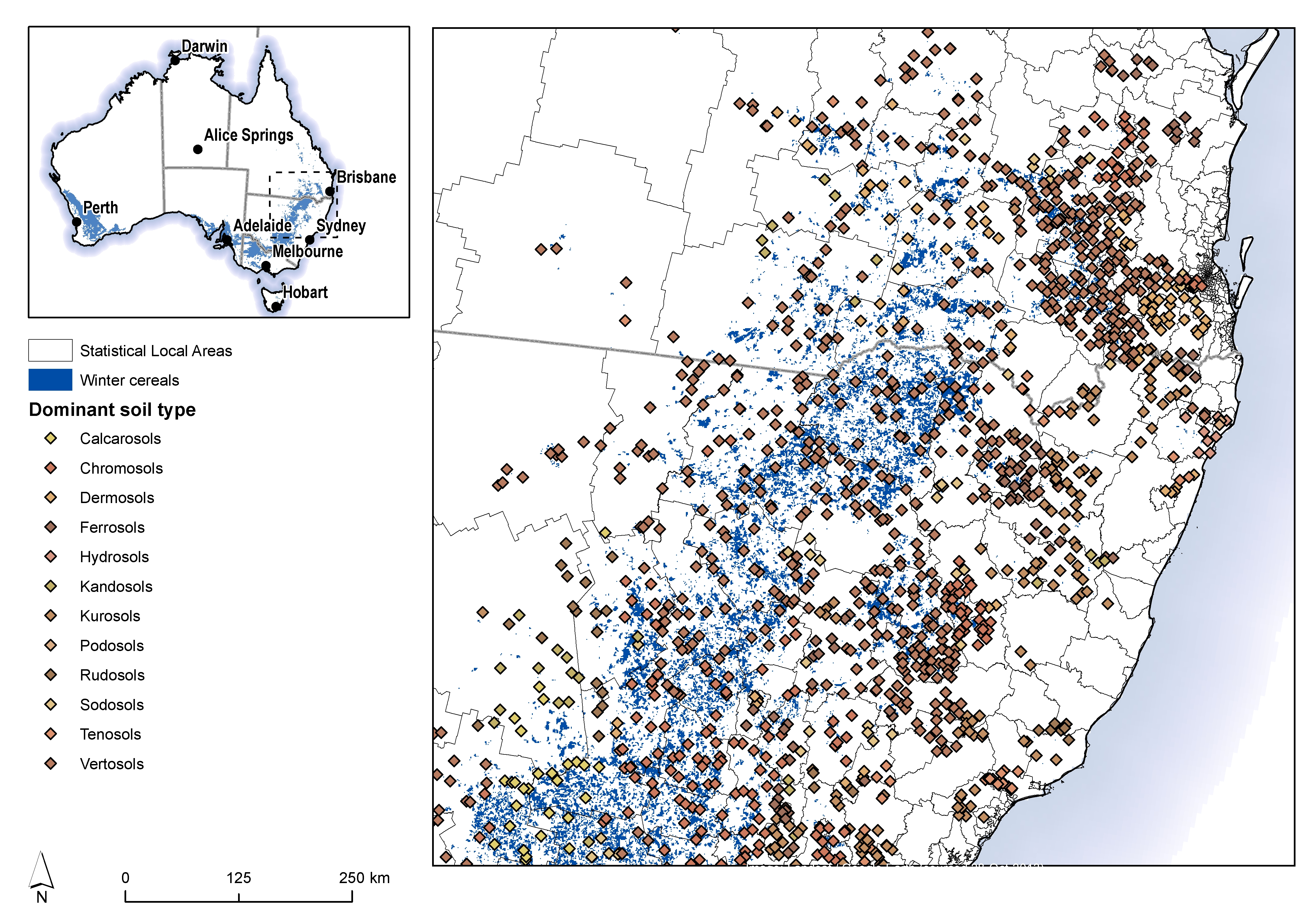
Figure 2 text description:  The dominant soil types found were calcarosols, chromosols, dermosols, ferrosols, hydrosols, kandosols, kurosols, podosols, rudosols, sodosols, tenosols and vertosols. Areas were marked for winter cereals of left for statistical local areas. The region tested extended just north of Brisbane and finished just before Sydney with the coast in the region and reaching far inland. Winter cereals were more inland away from the coast but ran parallel to the coast and lessened the further north the region went past Brisbane. The dominant soil type that was mainly found around Brisbane was vertosols. Chromosols and podosols soil type was also found in the Brisbane area but not in as large areas. The same soil mix was found similarly down the coast. Vertosols were found inland as well but not in as high areas as at the coast. In the furthest south west region the dominant soil type was calcarosols. The central south region saw a dominant soil type of chromosols and kurosols.

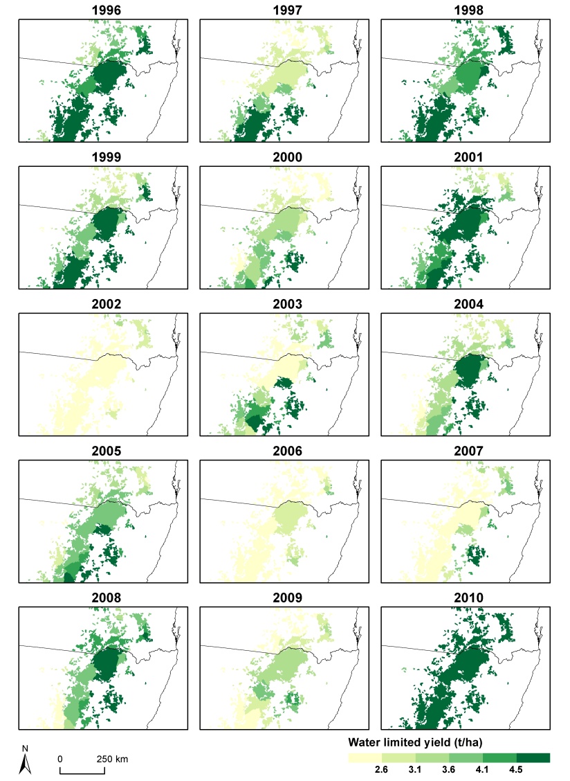
Figure 3 text description:

• In 1996, the central region showed a water limited yield of approximately 4.6t/ha. The northern region showed a yield of approximately 3.1t/ha in the north west to approximately 4.6t/ha in the north east. The southern region showed a yield of mostly around 4.6t/ha but reached a low of approximately 3.0t/ha in the south west.
• In 1997, the central region showed a water limited yield of approximately 3.0t/ha. The northern region showed a yield of approximately 2.5t/ha but reached up to approximately 3.0t/ha in the north east. The southern region showed a yield of approximately 3.2t/ha in the south west to approximately 4.6t/ha in the south east.
• In 1998, the central region showed a water limited yield of approximately 4.3t/ha. The northern region showed a yield of approximately 3.8t/ha in the north west to approximately 4.6t/ha in the north east. The southern region showed a yield of approximately 4.6t/ha.
• In 1999, the central region showed a water limited yield of approximately 4.6t/ha. The northern region showed a yield that decreased the further north the region became to approximately 2.8t/ha. The southern region showed a yield that increased the further south the region became to approximately 4.6t/ha.
• In 2000, the central region showed a water limited yield of approximately 3.3t/ha. The northern region showed a yield of approximately 2.6t/ha. The southern region showed a yield ranging from approximately 2.5t/ha to approximately 4.5t/ha in the south east.
• In 2001, the central region showed a water limited yield of approximately 4.6t/ha. The northern region showed a yield that decreased the higher the region became to a low of approximately 2.7t/ha. The southern region showed a yield of approximately 3.6t/ha in the south west to approximately 4.6t/ha in the south east.
• In 2002, all regions showed a water limited yield of approximately 2.5t/ha with it reaching approximately 3.0t/ha in the north east and south east.
• In 2003, the central region showed a water limited yield of approximately 2.5t/ha. The northern region showed a yield of approximately 2.5t/ha in the north west to approximately 3.7t/ha in the north east. The southern region showed a yield of approximately 3.2t/ha in the south west to approximately 4.6t/ha in the south east.
• In 2004, the central region showed a water limited yield of approximately 4.6t/ha. The northern region showed a yield of approximately 3.4t/ha. The southern region showed a yield of approximately 3.1t/ha in the south west to approximately 4.6t/ha in the south east.
• In 2005, the central region showed a water limited yield of approximately 3.7t/ha. the northern region showed a yield of approximately 3.4t/ha. The southern region showed a yield of approximately 3.1t/ha in the south west to approximately 4.5t/ha in the south east.
• In 2006, the central region showed a water limited yield of approximately 2.9t/ha. The northern region showed a yield of approximately 2.5t/ha but reached approximately 3.2t/ha in the north east. The southern region showed a yield of approximately 2.5t/ha but reached approximately 3.1t/h in the south east.
• In 2007, the central region showed a water limited yield of approximately 2.5t/ha. The northern region showed a yield of approximately 2.5t/ha in the north west to approximately 3.7t/ha in the north east. The southern region showed a yield of approximately 2.5t/ha in the south west to approximately 4.6t/ha in the south east.
• In 2008, the central region showed a water limited yield of approximately 4.6t/ha. The northern region showed a yield of approximately 3.6t/ha to 4.3t/ha. The southern region showed a yield of approximately 2.6t/ha in the south west to approximately 4.6t/ha in the south east.
• In 2009, the central region showed a water limited yield of approximately 3.4t/ha. The northern region showed a yield of approximately 2.5t/ha but reached approximately 3.5t/ha in the north east. The southern region showed a yield of approximately 2.5t/ha in the south west to approximately 4.2t/ha in the south east.
• In 2010, all regions showed a water limited yield of approximately 4.6t/ha.

Figure 4. Wheat yield gaps in Australia’s northern grain zone (aggregated at SLA level)

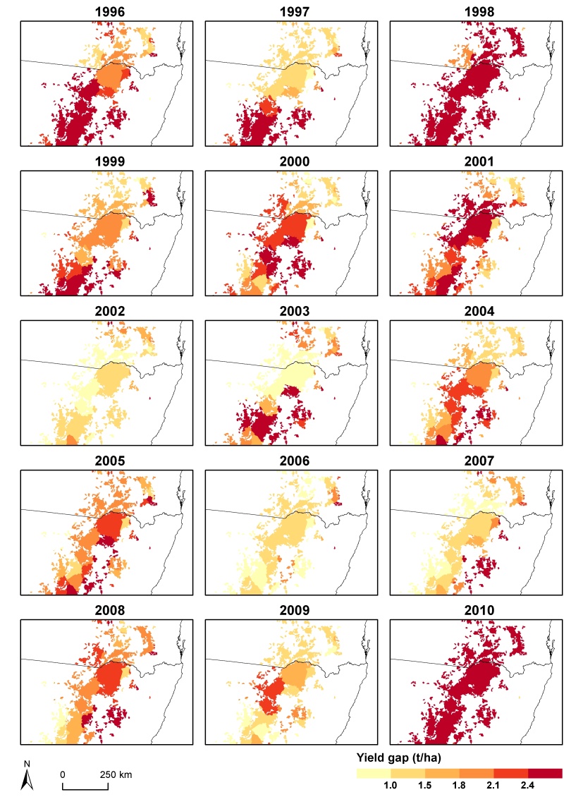
Figure 4 text description:

• In 1996, the central region showed a yield gap of approximately 2.9t/ha. The northern region showed a yield gap of approximately 1.8t/ha reaching up to approximately 2.4t/h in the far north. The southern region showed a yield gap of approximately 2.5t/ha.
• In 1997, the central region showed a yield gap of approximately 1.3t/ha. The northern region showed a yield gap of approximately 1.3t/ha. The southern region showed a yield gap of approximately 2.5t/ha.
• In 1998, all regions showed a yield gap of approximately 2.5t/ha with the yield gap reaching approximately 2.1t/ha in the west.
• In 1999, the central region showed a yield gap of approximately 1.9t/ha. The northern region showed a yield gap of approximately 1.4t/ha reaching approximately 2.5t/ha in the north east. The southern region showed a yield gap of approximately 1.8t/ha reaching to approximately 2.5t/ha in the far south.
• In 2000, the central region showed a yield gap of approximately 2.3t/ha. The northern region showed a yield gap of approximately 1.5t/ha. The southern region showed a yield gap of approximately 1.5t/ha reaching to approximately 2.5t/ha in the south east.
• In 2001, the central region showed a yield gap of approximately 2.5t/ha. The northern region showed a yield gap of approximately 2.1t/ha. The southern region showed a yield gap of approximately 1.7t/ha to approximately 2.5t/ha.
• In 2002, the central region showed a yield gap of approximately 1.2t/ha. The northern region showed a yield gap of approximately 0.9t/ha in the north west to approximately 1.5t/ha in the north east. The southern region showed a yield gap of approximately 1.4t/ha.
• In 2003, the central region showed a yield gap of approximately 0.9t/ha. The northern region showed a yield gap of approximately 0.9t/ha to approximately 2.4t/ha. The southern region showed a yield gap of approximately 1.8t/ha to approximately 2.5t/ha.
• In 2004, the central region showed a yield gap of approximately 2.0t/ha. The northern region showed a yield gap of approximately 1.5t/ha. The southern region showed a yield gap of approximately 1.0t/ha in the south west to approximately 2.5t/ha in the south east.
• In 2005, the central region showed a yield gap of approximately 2.3t/ha. The northern region showed a yield gap of approximately 2.0t/ha reaching approximately 2.5t/ha in the north east. The southern region showed a yield gap of approximately 1.5t/ha to approximately 2.5t/ha.
• In 2006, the central region showed a yield gap of approximately 1.3t/ha. The northern region showed a yield gap of approximately 0.9t/ha in the north west to approximately 2.1t/ha in the north east. The southern region showed a yield gap of approximately 0.9t/ha in the south west to approximately 1.6t/ha in the south east.
• In 2007, the central region showed a yield gap of approximately 1.3t/ha. The northern region showed a yield gap of approximately 0.9t/ha in the north west to approximately 2.3t/ha in the north east. The southern region showed a yield gap of approximately 0.9t/ha in the south west to approximately 2.5t/ha in the south east.
• In 2008, the central region showed a yield gap of approximately 2.3t/ha. The northern region showed a yield gap of approximately 1.5t/ha to approximately 2.2t/ha. The southern region showed a yield gap of approximately 1.0t/ha in the south west to approximately 2.5t/ha in the south east.
• In 2009, the central region showed a yield gap of approximately 1.7t/ha. The northern region showed a yield gap of approximately 1.3t/ha. The southern region showed a yield gap of approximately 1.0t/ha to approximately 2.1t/ha.
• In 2010, all regions showed a yield gap of approximately 2.5t/ha.

Figure 5. Correlation yield gap with water limited yield. Each value is based on 15 year means of SLA data. Data from 259 SLAs are included in the analysis. 

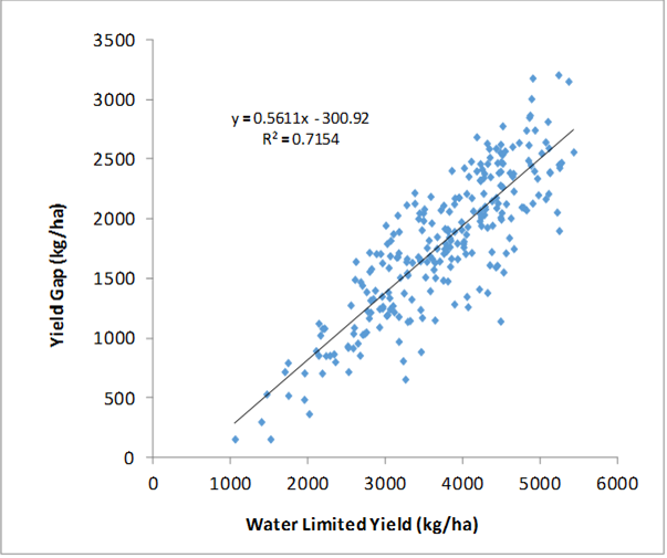
Figure 5 text description: There was a clear increasing trend between yield gap and water limited yield. As the yield gap increased, so did the water limited yield. It was found that 71.54% of the increase in yield gap could be attributed to the increase in water limited yield.

Figure 6. Relative wheat yields in Australia’s northern grain zone (aggregated at SLA level)

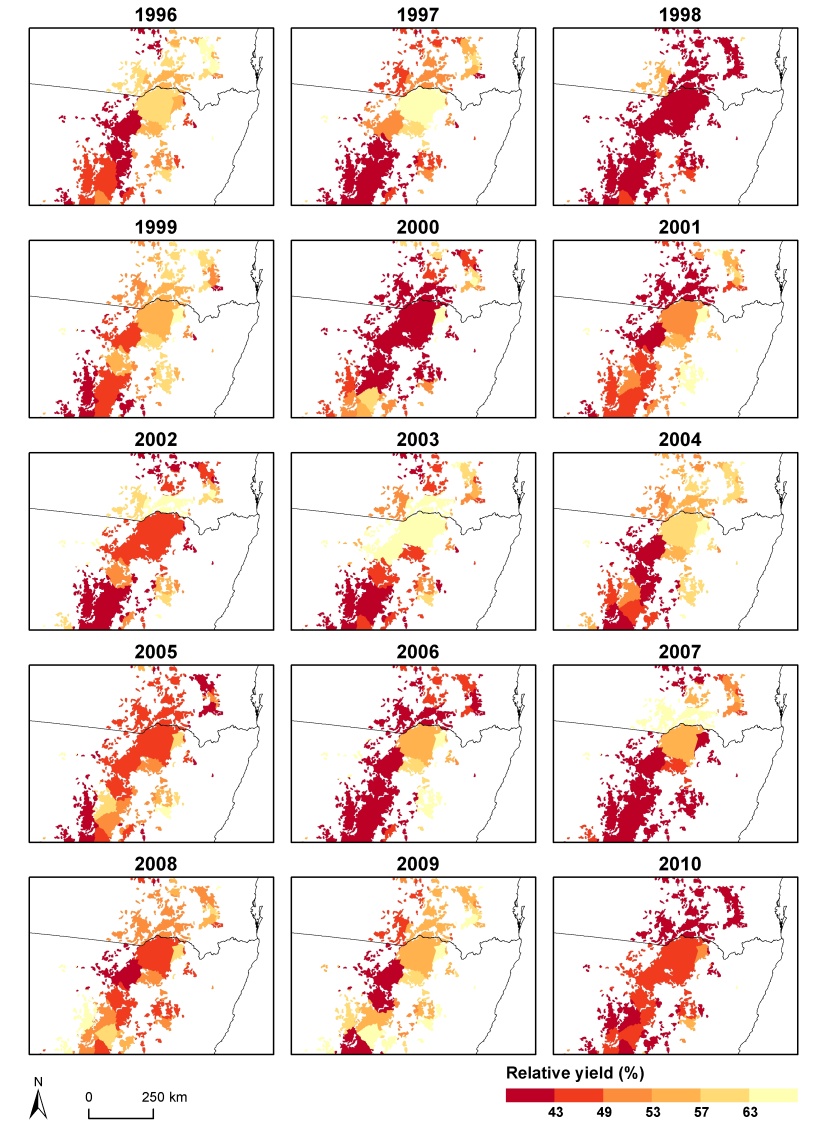
Figure 6 text description:

• In 1996, the central region showed a relative yield of approximately 60%. The northern region showed a relative yield ranging from approximately 42% in the north west to approximately 63% in the north east. The southern region showed a relative yield of approximately 42% in the south west to approximately 55% in the south east.
• In 1997, the central region showed a relative yield of approximately 64%. The northern region showed a relative yield of approximately 45% in the north west to approximately 57% in the north east. The southern region showed a yield of approximately 42%.
• In 1998, all regions showed a relative yield of approximately 42% with one spot reaching to approximately 50%.
• In 1999, the central region showed a relative yield of approximately 55%. The northern region showed a relative yield of approximately 57%. The southern region showed a relative yield of approximately 42% in the south west to approximately 60% in the south east.
• In 2000, the central region showed a relative yield of approximately 42%. The northern region showed a relative yield of approximately 43% in the north west to approximately 54% in the north east. The southern region showed a relative yield of approximately 42% reaching to approximately 56% in the furthest south.
• In 2001, the central region showed a relative yield of approximately 51%. The northern region showed a relative yield of approximately 42% in the north west to approximately 56% in the north east. The southern region showed a relative yield of approximately 42% in the south west to approximately 64% in the south east.
• In 2002, the central region showed a relative yield of approximately 46%. The northern region showed a relative yield of approximately 42% to approximately 63%. The southern region showed a relative yield of approximately 42% in the south west to approximately 58% in the south east.
• In 2003, the central region showed a relative yield of approximately 64%. The northern region showed a relative yield of approximately 43% to approximately 63%. The southern region showed a relative yield of approximately 42% in the south west to approximately 57% in the south east.
• In 2004, the central region showed a relative yield of approximately 57%. The northern region showed a relative yield of approximately 57%. The southern region showed a relative yield of approximately 43% in the south west to approximately 60% in the south east.
• In 2005, the central region showed a relative yield of approximately 45%. The northern region showed a relative yield of approximately 45% reaching to approximately 42% in the north east. The southern region showed a relative yield of approximately 42% in the south west to approximately 60% in the south east.
• In 2006, the central region showed a relative yield of approximately 51%. The northern region showed a relative yield of approximately 42% to approximately 48%. The southern region showed a relative yield of approximately 42% in the south west to approximately 64% in the south east.
• In 2007, the central region showed a relative yield of approximately 53%. The northern region showed a relative yield of approximately 42% to approximately 64%. The southern region showed a relative yield of approximately 42%.
• In 2008, the central region showed a relative yield of approximately 45%. The northern region showed a relative yield of approximately 51%. The southern region showed a relative yield of approximately 49% in the south east to approximately 63% in the south west.
• In 2009, the central region showed a relative yield of approximately 55%. The northern region showed a relative yield of approximately 45% in the north west to approximately 63% in the north east. The southern region showed a relative yield of approximately 42% in the south west to approximately 64% in the south east.
• In 2010, the central region showed a relative yield of approximately 45%. The northern region showed a relative yield of approximately 42%. The southern region showed a relative yield of approximately 42% to approximately 50%.

Figure 7. Wheat yields and yield gaps in the northern grain zone – 15 year SLA averages (1996-2010)

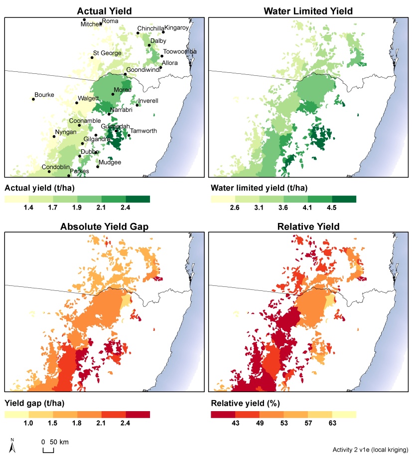
Figure 7 text description:

• The central region showed an actual yield of approximately 2.0t/ha. The northern region showed an actual yield of approximately 1.3t/ha in the north west to approximately 2.0t/ha in the north east. The southern region showed an actual yield of approximately 1.4t/ha in the south west to approximately 2.5t/ha in the south east.
• The central region showed a water limited yield of approximately 3.8t/ha. The northern region showed a water limited yield of approximately 2.6t/ha in the north west to approximately 4.2t/ha in the north east. The southern region showed a water limited yield of approximately 3.0t/ha in the south west to approximately 4.6t/ha in the south east.
• The central region showed an absolute yield gap of approximately 2.0t/ha. The northern region showed a yield gap of approximately 1.8t/ha. The southern region showed a yield gap of approximately 1.5t/ha in the south west to approximately 2.5t/ha in the south east.
• The central region showed a relative yield of approximately 51%. The northern region showed a relative yield of approximately 43% to approximately 57%. The southern region showed a relative yield of approximately 42% in the south west to approximately 56% in the south east.

Table 1. Yield Gap results for the GRDC regions – 15 year (1996-2010) area weighted average values

^# of the 259 SLAs  used in the national analysis 31 fall outside GRDC regions

Conclusion

The key observation from this analysis of wheat crop yields is that over the period from 1996 to 2010 there was an average yield gap of 1.9 t/ha in the northern region. Relative to the average water limited yield of 3.6 t/ha, the average actual yield of 1.7 t/ha was 46.6%. If we accept that farmers can sustainably achieve a relative yield of 80%, as was demonstrated by leading farmers in the Wimmera and Mallee (van Rees et al. in review), then this study suggests that farmers in the northern region could achieve average yields of 2.9 t/ha or that there is scope to close the exploitable yield gap and increase average yields by 1.2 t/ha.

The northern region’s relative yields of 46.6% were 5.3% lower than relative yields in the southern region and 8.9% lower than in the western region. Hence there is more scope to boost yields in the northern region through better application of current technologies and best practice.

Individual farmers and their advisers need to focus more closely on their own yields relative their farms’ location. Are they achieving better or worse than their SLA’s average yields over the same period? How close are they to closing the exploitable yield gap and consistently achieving a relative yield of 80%? Advisers will be interested to know how close their best clients are to Yw and how much of a gap there is still there for them to exploit. If the answer is not much then these farmers will need to pioneer new technology breakthroughs to improve their yields. Advisers should also challenge themselves to diagnose the cause of the yield gap for those clients who have large exploitable yield gaps.

In the next few months we will develop a website in which farmers and advisers will be able to zoom into their farm location and obtain an instant benchmark relative to Ya, Yw, Yg and Y_%. We are keen to test the usability and usefulness of this website with farmers and advisers. If you are keen to be among the first to test drive the system and help guide its development please contact me after the break.

References

ABARE–BRS, 2010. Land Use of Australia, Version 4, 2005–06 dataset.

ABS, 2009. ABS Agriculture Statistics Collection Strategy – 2008–09 and beyond,

2009. Cat. no. 7105.0

Alexandratos, N., Bruinsma, J. 2012. World agriculture towards 2030/2050: the 2012 revision. ESA Working paper No. 12-03. Rome, FAO.

Bryan, B.A., Barry, S., Marvanek, S., 2009. Agricultural commodity mapping for land use change assessment and environmental management: an application in the Murray–Darling Basin, Australia. J. Land Use Sci. 4 (3), 131–155.

Evans, L.T., Fischer, R.A. 1999.  Yield potential: its definition, measurement and significance.  Crop Sci. 39, 1544-1551.

Patricio Grassini, Kent M. Eskridge, Kenneth G. Cassman., 2013. Distinguishing between yield advances and yield plateaus in historical crop production trends. Nature Communications. 4:2918. DOI: 10.1038/ncomms3918.

Hochman, Z., Holzworth, D.P., Hunt J.R., 2009. Potential to improve on-farm wheat yield and water-use efficiency in Australia. Crop Pasture Sci. 60, 708-716.

Hochman, Z., Gobbett, D., Holzworth, D., McClelland, T., van Rees, H., Marinoni, O., Garcia, J.N., Horan, H., 2012. Quantifying yield gaps in rainfed cropping systems: a case study of wheat in Australia. Field Crops Res. 136, 85-96.

Lobell, D.B., Cassman, K.G., Field, C.B., 2009. Crop yield gaps: Their importance, magnitudes and causes. Ann. Rev. Environ. Resour. 34, 179-204.

van Ittersum, M.K., Cassman, K.G, Grassini, P., Wolf, J., Tittonell, P., Hochman, Z., 2013. Yield gap analysis with local to global relevance—A review. Field Crops Res. 143, 4–17.

Harm van Rees, Tim McClelland, Zvi Hochman, Peter Carberry, James Hunt, Neil Huth, Dean Holzworth, 2014. Leading farmers in South East Australia have closed the exploitable wheat yield gap: simulation for benchmarking and exploring options for increased production. In review.

Contact details

Ph: 07 3833 573307 3833 5733 07 3833 573307 3833 5733