We can monitor soil moisture content - now what?
Author: Neil Huth, Tim McClelland, Harm van Rees and Bill Long | Date: 05 Feb 2014
Neil Huth1, Tim McClelland2, Harm van Rees3 and Bill Long4
1CSIRO, 2BCG, 3Crop Facts, 4AgConsulting Co.
Take home messages
- Soil moisture probes provide easily understood outputs of soil water.
- Yield Prophet®, using APSIM modelling, simulates soil water, crop water use and nitrogen (N) use on a daily basis and provides a risk assessment, through probability, of achieving a target yield.
- Integrating modelling and monitoring can provide a means to simultaneously improve both. This could potentially include calibration of probes and Yield Prophet® at the same time.
- While the focus of the interest has been directed towards the integration soil moisture probes with models the integration of weather station data also has a significant contribution to make to improve model accuracy.
Comparing soil water information presented by probes and Yield Prophet®
Over recent years there has been significant interest in capacitance soil moisture probes fitted with weather stations for monitoring crop water availability and climatic conditions in crop. Model supporters are challenged by the interest in probe use by farmers and some advisors when models (e.g. Yield Prophet®) have been doing the same for longer and for a fraction of the cost. The way in which soil water information is presented by probes and Yield Prophet® is very different. There are pros and cons associated with both systems. The type of information provided by soil moisture probes and Yield Prophet® are detailed in Figures 1 and 2, including comments on each method.
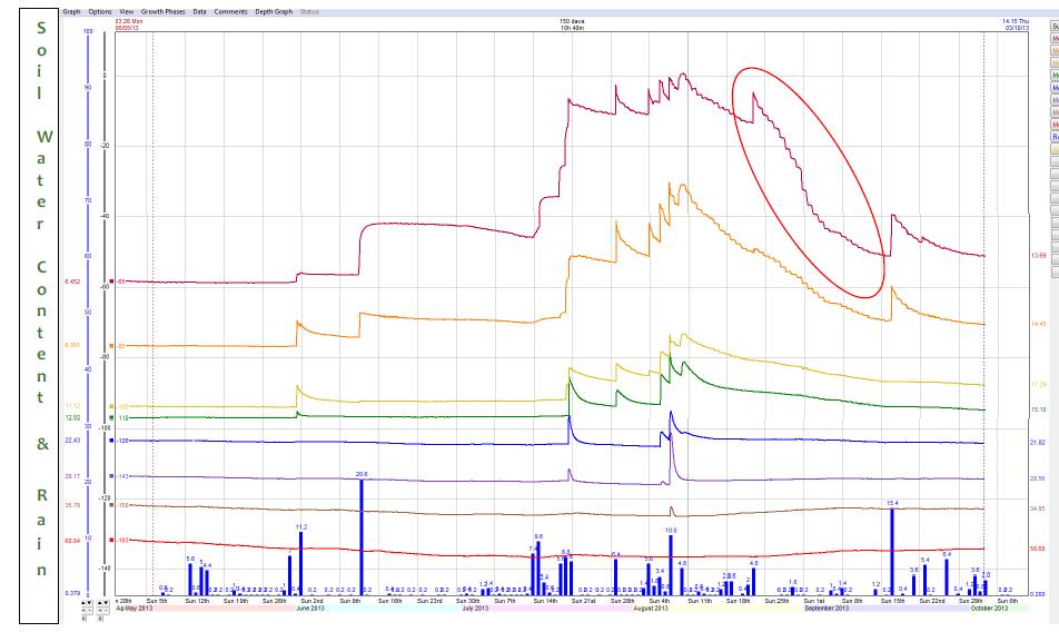
Comments:
- shows total soil water and increase in soil water following rain
- dry period during Aug-Sep depleted most of the available stored water (period circled on the graph)
- shows limit to plant water use at 60cm (rooting depth)
- estimate of crop lower limits (CLL) at the end of this cropping season (after a long dry spell)
- note drained upper limit (DUL) was probably not achieved; and
- uses a generic calibration for calculating volumetric soil water.
Figure 1. Typical soil moisture probe data representation for a wheat crop, May to October 2013. Lines are soil moisture content (mm) at eight depths in the profile (shallowest 30cm; deepest 100cm). Bars are rainfall (mm).
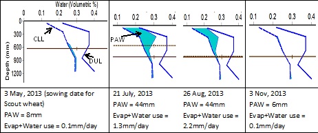
Comments:
- CLL and DUL from soil characterisation (users have access to a large Australia-wide data base of characterised soils)
- plant available water (PAW) highlighted on the graph and listed as an output in mm
- daily water balance as simulated from the time of soil sampling (pre-sowing)
- daily water use provided, and
- water stress exhibited by the crop expressed in another graph.
Figure 2. APSIM modelled plant available water as represented by Yield Prophet® for a wheat crop in 2013.
The fact that soil moisture probes can be held and be touched has meant that growers are comfortable with the data being produced. While probe data has many benefits, the practical application of the output data is limited. Often it is difficult to quantify the amount of soil moisture available to a crop because of the absence of meaningful data about the water-holding capacity of the soil. Further to this, applying the data to a decision can be difficult. The benefit of the data comes from integration with other decision support systems.
Yield Prophet® and soil moisture probes – where are we and where too from here?
At present, Yield Prophet® crop simulations are created by combining the essential components of growing a crop including:
- a soil test sampled prior to planting
- a soil classification selected from the APSoil library of approximately 1,000 soils selected as representative of the production area
- historical and recent climate data taken from the nearest Bureau of Meteorology (BOM) weather station
- paddock specific rainfall data recorded by the user (optional)
- individual crop details (e.g. cultivar, sowing date), and
- fertiliser and irrigation applications during the growing season.
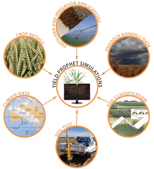
Figure 3. Yield Prophet simulation inputs.
During the 2012 season, Yield Prophet® was amended to enable soil moisture probe data and climate data to feed directly into the program. This involves probe data being sent to a central location from which Yield Prophet® can collect the data. The initial phase of this process has focused on outputting the soil moisture probe data next to simulated soil moisture data from APSIM. This initial phase allows the two systems to be viewed side by side where they can act as validation for each other. The validation may assist users of both systems in identifying faulty readings on the probes and incorrect outputs from the simulations.
Figure 4 shows one of the outputs from the new Yield Prophet® soil probe crop report. The output is showing the probe (‘Probe’) and the simulated (‘Virtual’) soil water values from the summed profile (Total) and individual sensor depths (e.g. 10cm). It is evident from the figure that, in this example, the absolute values returned from the two systems are different but show a consistent offset. In this case the two systems are acting as a positive validation, but it is clear that the calibration of the probe water values need to be adjusted so as to more closely reflect the simulated values or vice versa.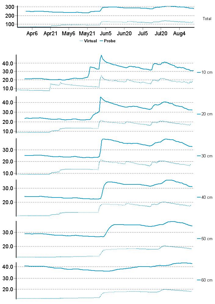
Figure 4. Probe (solid line) and simulated/virtual (dotted line) plant available water at different depths and a summed total from the new Yield Prophet® soil probe crop report.
The second phase of incorporating the two systems could involve feeding probe data into APSIM and allowing APSIM to generate crop simulations based on this data. However, before this can occur, further research is required to determine whether this is possible.
So, how would we go about marrying models and measurements?
This area has had a lot of coverage in the scientific literature as models are increasingly used to inform decisions and as real time data becomes more readily available. The problem is often referred to as data assimilation (DA) or model-data fusion. One of the most common uses is in informing large scale spatial simulations through the use of remote sensing, most commonly satellite imagery. In these cases, surface spectral properties are used to infer surface conditions, such as vegetation cover, which are then used as an input into the simulation. This means that modellers operating at a global scale do not need to know everything about every crop in every paddock.
There are three main ways to assimilate models and data (Dorigo et al 2007):
- Forcing method: the state variable in the model is directly replaced by the measured data. This requires continuous information on the time step used by the model.
- Calibration method: model inputs or initial conditions are adjusted to create optimal agreement between the model and the observed data. This can require a large amount of computing time.
- Updating method: the model is sequentially updated whenever an observation is required.
If done carefully, and correctly, any of the above can be used in the example of the use of satellite imagery for informing modelling of canopy development. In this case, an estimate of crop cover (from spectral indices) can be used to constrain the model so that modelled growth more closely matches that observed in the field. In this case, the data used to constrain the model may be a driver of the output of interest but with little feedback from that output of interest. In the case of soil moisture sensors, things are slightly different.
Two ideas are important. Firstly, in rain-fed environments, production is closely driven by water supply; any error in crop water use will likely impact on yield prediction. However, errors in water supply are constrained by the fact that water use cannot exceed water supply (i.e. effective rainfall + stored soil moisture). Therefore, better information on soil water supply should improve yield predictions. Conversely, any information or method that adversely impacts water balance predictions will harm yield predictions. This leads to the second point.
We need to recognise that nothing is perfect. There are errors in our model, for example. For this reason, we look to incorporate measured data into the model (i.e. to reduce error). However, the measured data is also imperfect. Direct incorporation of imperfect data into an already imperfect model may in fact increase model error. In Figure 5, we show soil water measured at various depths using gravimetric methods and EnviroSCAN™ probes at Norwin in Queensland during 2010 - 2012 (Dalgliesh 2013). We see large variation in gravimetric samples even though sampling with 12 replicate cores was used. Periods of equipment failure are evident in the EnviroSCAN™ data. Finally, discrepancy between the various measured and modelled time series are not insignificant. It is not clear that constraining the model using either of the observed datasets would actually improve yield estimations.
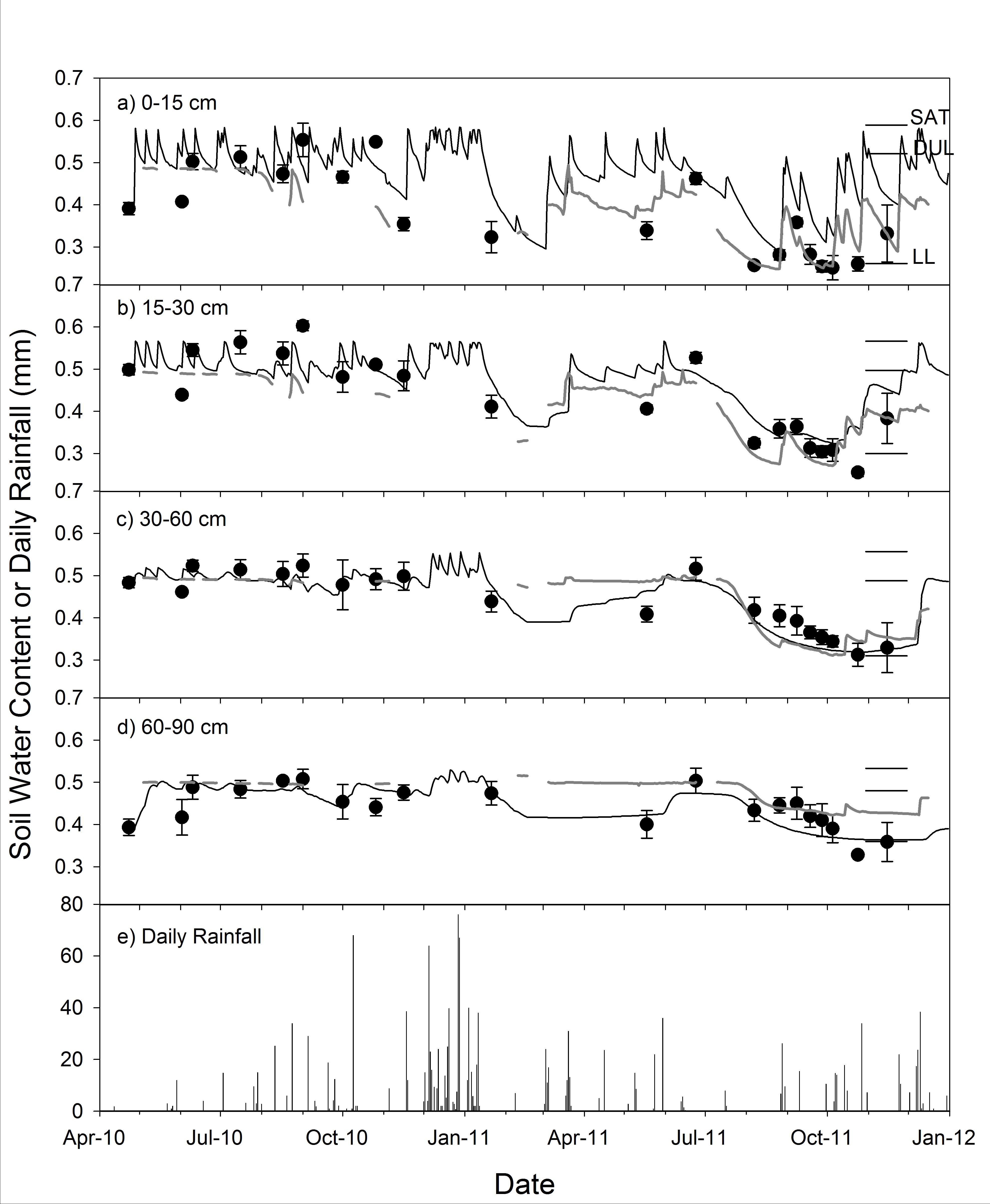
Figure 5. Time series of measured gravimetric (circles), EnviroSCAN™ measured (thick line) and APSIM-simulated (thin line) soil water at Norwin during 2010 to 2012.
Furthermore, the mere act of interfering with the model can exacerbate errors within the model. Correcting prediction errors in a major driver of the system (i.e. soil water) without also correcting other prediction errors arising from that error (e.g. an overestimation in growth) can destroy compensating errors that restrict the model from diverging from reality. For example, consider the case where water use is over-predicted, resulting in over-predictions of growth. Correcting the soil water content without correcting the growth will simply result in increasing water supply for the next day, which will likely result in even more accelerated growth. Total water use for the season will be accidentally inflated, errors in growth are never corrected, and model predictions are likely to be worse than if they were not 'corrected'. This sort of adverse impact is likely for the forcing and updating methods.
The short message is this, simple combinations of models and observed data are likely to decrease predictive capacity through:
- introducing new error into model parameterisation
- additive errors when combining imperfect models and imperfect data, or
- destroying compensating errors within the model.
So what is the answer?
There are methods that can help with all these problems. These are often referred to as filtering techniques in that they filter out bad data or model parameterisations and provide estimates of the confidence you should have in both models and the data. These techniques also arise out of the aerospace industries, where the earliest approaches were developed for reducing errors in predictions of missile or spacecraft positions estimated from measurements of speed and direction. Measurements in the movement of spacecraft have errors and predictions are affected by these. Filtering techniques were developed to pull the 'noise' out of the measurements to improve predictions.
The really good news is that methods used in assimilating models and soil moisture probes could be used to improve the quality of the information from the model, and also the quality of information from the probes. It is clear that probe data can help identify when the model is correct or incorrect. It is also possible that such techniques would allow the model to help identify periods when the probes are not working correctly, or are not calibrated correctly. Take this simple example, a simple water balance model can tell you that there is a problem if probes register a jump in soil water content of 40 mm for a 20 mm rainfall event. Filtering techniques would provide a more powerful way of detecting these, and possibly suggesting likely causes of the problem. In essence, you may be able to calibrate your model and your sensors at the same time by having them learn from each other. In fact, it is not hard to imagine a system where model-data fusion is used to provide rapid estimates of probe calibration curves to improve the quality of data from probe networks.
So, the data assimilation could provide:
- a better parameterisation of the model
- better predictions from the model
- a better way to test sensor data, including indication of periods of lower data integrity (i.e. when to believe them or not), and
- another way to calibrate your sensors by accumulating information over time.
However, to do this requires:
- More computing power. Computing clusters will need to run large numbers of simulations to get enough information to find solutions to the problems. Yield prophet® already uses such clusters
- More sensors, information on uncertainty in sensor data helps here. This means replication of sensors.
- Better mathematics and more software behind the scenes than currently used in Yield Prophet®.
Key developments
While the focus of the interest has been directed towards integrating soil moisture probes with models, the integration of weather station data also has a significant contribution to make to improve model accuracy and reducing the effort associated using them effectively. At present Yield Prophet® uses climate information from the SILO Patched Point Dataset (PPD). This is a catalogue of climate information for 4,600 weather stations across Australia. Alternatively, users may enter rainfall for each paddock into the web interface. Currently users select a weather station from the database that is representative of the location of their paddock. The weather station has two distinct purposes in the simulations process:
- It provides climate data for the current season which is used to simulate crop growth and the soil water and nitrogen processes in the paddock from the time of soil sampling to the time of the report.
- It provides historic data which is used to simulate crop growth and resource availability from the day on which the report was generated to the end of the season. This process is repeated once for each year of climate record (approx. 120 years) providing 120 separate yield outcomes.
While this system is effective, there are some situations where the chosen weather station is a significant distance away from the paddock being simulated. Australia’s climate is highly variable and small distances can result in large differences in the climate between the weather station and the paddock of interest. This is especially the case for minimum air temperatures where local topography can cause substantial differences (Figure 6).
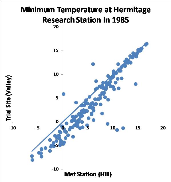
Figure 6. Plot of daily minimum air temperature (°C) for Hermitage Research Station, Qld, in 1985, comparing temperatures at the base of a small valley to those at a met station on a hill side.
These differences can cause quite large model error. This error can be reduced by having live weather stations located in the paddock being simulated. However, it should be noted that this improvement will only be realised in the simulation of crops in the current season. Yield Prophet® will still need to use the historic records from the PPD as the basis for simulations from the day on which the report was generated to the end of the season.
Table 1 shows some key outputs from two reports, generated on the same day for the same paddock. The only difference between the two is the source of climate data. Report 1 used the current Yield Prophet® system, where temperature was sourced from SILO and rainfall from the farmer’s rain gauge. Report 2 used the probe weather station for both rainfall and temperature. It is evident from the table that Report 1 had a significantly higher yield potential, had more rainfall recorded and was at an earlier growth stage. In this situation Report 1 was closer to reality.
Upon investigation, it became apparent that the probe weather station had stopped recording rainfall for a period. Furthermore, it was not equipped with a temperature sensor housed in a Stevenson screen. The temperature sensor was housed with the data logging unit. As such, the temperature readings were several degrees higher than reality. As a result, the simulated growth stages were well in advance of what was occurring in the paddock and this reduced the simulated yield potential. This example does not show a situation where the simulation has improved. However, it does show the potential benefits coming from integrating models and monitoring at a local scale. It also shows an example of how the two systems can be used to validate each other.
Table1. Yield potential, temperature and rainfall source, and simulated growth stage outputs from reports generated on the same crop on 12 August 21013
|
Item
|
Report 1
|
Report 2
|
|
Yield potential
|
|
|
|
|
||
|
Temperature source
|
Silo
|
Probe weather station
|
|
Rainfall source
|
Manually entered
(187.4mm)
|
Probe weather station
(150.7mm)
|
|
Growth stage
|
Mid booting
(GS45)
|
Early flowering
(GS62)
|

References
Dalgliesh N.P. (2013). Doing it better, doing it smarter-managing soil water in Australian agriculture. Final report on project CSA00023 to the Grains Research and Development Corporation, PO Box 5367 Kingston, ACT 2604 Australia, June 2013 http://www.grdc.com.au
Dorigo, W.A., Zurita-Milla, R., de Wit, A.J.W., Brazile, J., Singh, R., Schaepman, M.E. (2007). A review on reflective remote sensing and data assimilation techniques for enhanced agroecosystem modelling. International Journal of Applied Earth Observation and Geoinformation 9, 165-193.
Contact details
Tim McClelland
P.O. Box 85, 73 Cumming Ave, Birchip VIC, 3483
03 5492 2787
Neil Huth
PO Box 102. 203 Tor St, Toowomba QLD, 4350
07 4688 1421
Neil.Huth@csiro.au
Was this page helpful?
YOUR FEEDBACK