Farming practices that maximise water use efficiency
Author: James Hunt, John Kirkegaard, Claire Browne, Therese McBeath and Simon Craig | Date: 17 Jul 2012
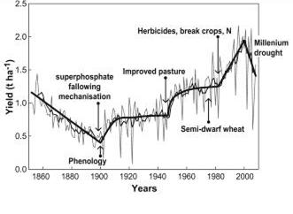
Figure 1. Trends in Australian average annual wheat
yields (line) and 10 yr moving average (bold).
The approximate timing of selected management (above
line) and breeding innovations (below line) are indicated
by arrows (taken from Kirkegaard and Hunt 2010).
James Hunt1, John Kirkegaard1, Claire Browne2, Therese McBeath3 & Simon Craig2
1CSIRO Sustainable Agriculture Flagship, 2Birchip Cropping Group, 3CSIRO Sustainable Agriculture Flagship
Keywords: water-use efficiency, summer fallow management, break crops, early sowing
Take home messages
- Good water-use efficiency comes from farming systems (not just new varieties, chemicals or fancy machinery!)
- Management decisions that are taken before a crop is planted (e.g. tillage system, summer fallow management, crop sequence) often have greater potential to improve water-use efficiency than in-crop management decisions
- In the Wimmera-Mallee, no-till, summer weed control, crop sequences that include a legume and early sowing are all practices that complement each-other and improve water-use efficiency
Improving water-use efficiency
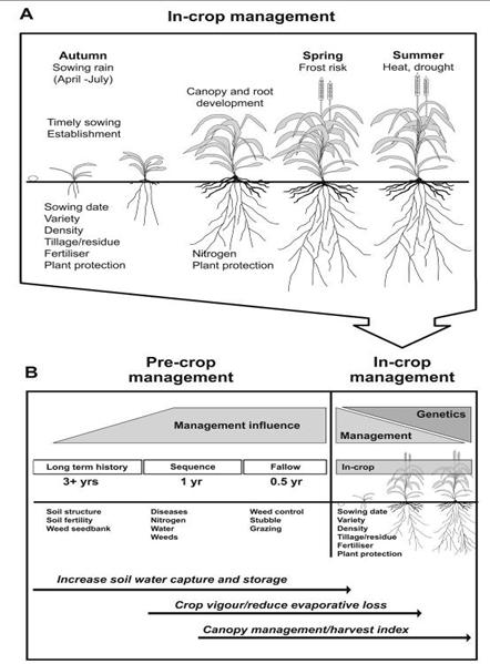
Figure 2. The range of in-crop management options (A) that influence the
productivity and water-use efficiency of cereal crops. Critical in-crop seasonal
influences at sowing, anthesis and maturity are shown. In-crop management
effects are placed in the context of various pre-crop management options (B),
and the continuum of overlapping influences of these various options on
components of water-limited yield are shown by horizontal arrows.
The history of Australian wheat production shows that major improvements in yield have occurred when a package of new genetic and/or management developments combine into an effective farming system (Figure 1).
In-crop and pre-crop management for water-use efficiency
Research into water-use efficiency often tends to focus on the in-crop period i.e. the period of time from when a crop is sown to when it is harvested (Figure 2A). However, management of farming systems during the pre-crop period often has greater potential to improve yield and profitability when water is limiting (Figure 2B).
A northern Victorian case study
To test the impact of farming systems on yields APSIM was used on a case study farm located near Kerang in northern Victoria. The comparisons represent the general farming system and evolution in management over the last 30 years of many progressive grain growing farms in low-rainfall regions of Australia. Six simulation scenarios (1962-2009) were created based on generalised progress in pre-crop and in-crop management made on the farm during the last 30 years (Table 1).
|
Scenario
|
Management Type |
|||||
|
Tillage system (pre-crop – long-term) |
Stubble (pre-crop-long-term) |
Summer weeds (pre-crop - fallow) |
Rotation (pre-crop – sequence) |
Sowing window (in-crop) |
Coleoptile (genetic) |
|
|
1. Baseline |
2 cultivations prior to sowing and full cut-out at sowing |
Burnt in Autumn |
No control until autumn |
Wheat-wheat |
21 May – 1 Aug |
Short |
|
2. Tillage system |
Direct drill, minimum till |
Fully retained |
No control until autumn |
Wheat-wheat |
21 May – 1 Aug |
Short |
|
3. Summer fallow |
Direct drill, minimum till |
Fully retained |
Full control |
Wheat-wheat |
21 May – 1 Aug |
Short |
|
4. Crop sequence |
Direct drill, minimum till |
Fully retained |
Full control |
Forage peas-wheat |
21 May – 1 Aug |
Short |
|
5. Sowing window |
Direct drill, minimum till |
Fully retained |
Full control |
Forage peas-wheat |
25 April – 1 Jul |
Short |
|
6. Genetic solution |
Direct drill, minimum till |
Fully retained |
Full control |
Forage peas-wheat |
20 April |
Long |
The case study scenarios
Scenario 1 (baseline) represents a conventional tillage farming system that was typical of regional practice until the late 1980s. Weeds are grazed by sheep over summer but not controlled, stubble is burnt in April and the paddock cultivated twice before being conventionally sown.
Scenario 2 (tillage system) represents the minimum till, retained stubble farming systems that developed during the 1980s. In this scenario, all stubble from the previous crop is retained until sowing. The sensitivity of the soil to run-off is reduced to reflect the better infiltration rates found in reduced tillage systems. In both Scenario 1 and 2, soil water is reset to the crop lower limit of wheat on 31 March each year to represent the situation where poor control of summer weeds used all the water that would otherwise have been available for subsequent crops.
In Scenario 3 (summer fallow) complete fallow weed control is practiced and all out-of-season rainfall not subject to evaporation is allowed to accumulate in the soil (Table 1). Scenarios 1, 2 and 3 involve a continuous wheat sequence, reflecting the cereal dominated crop sequences typical prior to the 1980s, and that have re-emerged in response to the millennium drought. Usually in this area, cereals use all of the plant available water in a given season and no residual water carries over to the next crop in the sequence.
In Scenario 4 (crop sequence), a forage field-pea crop cut for hay in October at early pod-set is introduced into the sequence. On the commercial farm, introduction of this crop in 2005 provided the case-study farm managers with a low risk break crop that remained profitable in dry years, and provided residual water that could be used by a wheat crop in the next season (many other farmers in the Wimmera-Mallee use vetch in a similar way). The aim here is not to compare the profitability of different crop sequences, but to quantify the impact that crop sequence has on subsequent crop yield. The disease, weed and nitrogen benefits of the break crop are not simulated so that yield increases in wheat are entirely due to additional water.
In Scenario 5 (sowing window), an earlier sowing window (25 April) is included to reflect the lowered risk afforded by sowing earlier into the stored soil water preserved by improved infiltration, fallow weed management, stubble retention and forage peas in the sequence.
In Scenario 6 (genetic solution), a novel genetic adaption -a wheat cultivar with a long coleoptile that could be sown deeply (a depth of 110 mm is used in the simulation) into soil water remaining from the previous field-pea crop and fallow period. This trait allows sowing on a calendar date, as soil water to germinate the crop is usually available at this depth in April, but is too deep for current short-coleoptile wheat varieties which need an opening rain to germinate and emerge. This trait would give greater control over the timing of crop emergence and maturity and optimise flowering time and thus yield potential for a given environment.
In order to demonstrate that individual management changes have greater impact when they form part of a coherent system, each of the management changes were also simulated individually and compared to the baseline scenario (Scenario 1).
All simulations were set up such that nitrogen availability did not limit yield. As APSIM does not model the negative effects on crop growth of weeds, pests, diseases, frost and heat, the yield values reported here are water-limited attainable yields. That is, yields which could be achieved by growers given skilful use of available technology and ignoring constraints placed on realised farm yields by operational considerations and input risk aversion.
Time of sowing in all simulations was determined by a threshold rainfall rule in which 15 mm or more must fall over a maximum of three days during the sowing windows specified in Table 1. A mid-early maturity wheat variety was used (e.g. Yitpi![]() , Correll
, Correll![]() ) and all crops were sown at a density of 150 plants/m2 and 21 cm row spacing.
) and all crops were sown at a density of 150 plants/m2 and 21 cm row spacing.
Impact of systems changes
Farming system changes introduced over the last 30 years have resulted in big improvements in yield and water-use efficiency (Table 2 and 3). The simulated change from the baseline scenario of full-tillage and no stubble retention to direct drill and stubble retention (Scenario 2) increased yield by a modest amount. This increase was due to a reduction in the proportion of run-off and evaporation relative to total water-use. The relatively small impact on yield, which did not improve in drier years, is consistent with the results of long-term experiments throughout southern Australia where tillage and stubble treatments were imposed under otherwise identical management, including sowing dates. This emphasises the fact that yield responses to reduced tillage and stubble retention alone may be small, or even negative, if synergistic changes to the system (e.g. sowing opportunities, summer weed control) as a whole are not considered.
Table 2. Mean simulated yield from the different scenarios for the years 1962-2009.
|
Scenario |
Management lever |
Mean grain yield (t/ha) |
|
1 |
Baseline |
1.6 |
|
2 |
Tillage system |
1.8 |
|
3 |
Summer fallow |
2.8 |
|
4 |
Crop sequence |
3.4 |
|
5 |
Sowing window |
4.0 |
|
6 |
Genetic solution |
4.5 |
Table 3. Mean increase in simulated yield assuming adaptations are added either sequentially or singularly. Numbers in brackets are the percentage increase relative to the mean yield of the baseline scenario (Table 2).
|
|
|
Mean yield increase - All years (t/ha) |
|
|
Scenario |
Management lever |
Additive |
Singular |
|
1 |
Baseline |
- |
- |
|
2 |
Tillage system |
0.2 (15) |
0.2 (15) |
|
3 |
Summer fallow |
1.0 (61) |
0.8 (49) |
|
4 |
Crop sequence |
0.6 (41) |
0.2 (10) |
|
5 |
Sowing window |
0.6 (36) |
0.5 (30) |
|
6 |
Genetic solution |
0.6 (36) |
-0.2 (-10) |
In contrast, the largest increase to yield and water-use efficiency was achieved by improved summer weed management (Scenario 3). This significantly increased water-use, and also improved water-use efficiency by increasing the average harvest index as more water was available to wheat crops available during spring. The yield increase is lower when fallow weed management was introduced alone (Table 3) because the soil cover and superior infiltration rates offered by stubble retention and minimum tillage are needed to maximise fallow efficiency.
The introduction of forage peas into the rotation (Scenario 4) also increased water carried over to the wheat crop and effectively acted in the same manner as summer weed management to improve yield. However, when added alone, the impact of the forage peas is much smaller because the water they leave is used by summer weeds and lost from bare, cultivated soil.
The ability to sow early (Scenario 5) increased yield significantly. However, sowing wheat dry or immediately after the autumn break is an adaptation only made possible by the exceptional weed control provided by the forage pea break crop, good fallow management and surface stubble from no-till extending the sowing window following marginal sowing rains.
A wheat variety with a long coleoptile gives a large yield increase in combination with the other management improvements (Scenario 6). However, this adaptation generates a yield decrease if added individually because in the absence of stored water from the pea crop, good fallow management and improved soil and stubble management, there is a yield penalty due to the time taken for the seed to emerge from depth after opening rains. This is a strong demonstration of how it can be counterproductive to develop and adopt new technologies if consideration is not given to how they might fit into the farming system as a whole.
Field trials support simulation case study
BCG and CSIRO have been researching the impact of summer fallow management and crop sequences at Hopetoun on two different soil types (sand and clay) as part of the GRDC National Water-use Efficiency Initiative. Over the three years of the experiments to date, they have found that controlling summer fallow weeds has dramatically increased yields by increasing both water and nitrogen available at sowing (Table 4). Return on investment in summer weed control over this period has averaged 377%. Retaining stubble vs. removing stubble or cultivating has only resulted in a small yield increase during one season (2012) at the sand site.
An experiment investigating the effect of different break crops (canola, peas and vetch vs. wheat-on-wheat and chemical fallow) and end-uses (grain, hay or brown manure) on wheat yield has found that including a legume in crop sequences increases the yield of subsequent wheat crops (Table 5) and overall profitability (Figure 3). Crop sequences involving canola were profitable because of the profitability of canola itself, rather than increases in wheat yield of subsequent crops (Table 5).
Table 4. Mean additional PAW, nitrogen, yield and return on investment ($/ha) from controlling summer weeds at both sites 2009-2011.
|
|
Sand |
Clay |
||||
|
|
2009 (barley) |
2010 (canola) |
2011 (wheat) |
2009 (barley) |
2010 (canola) |
2011 (wheat) |
|
Mean additional PAW at sowing (mm) |
26 |
40 |
29 |
10 |
52 |
36 |
|
Mean additional Nitrogen (kg N/ha) |
-5 |
45 |
41 |
10 |
44 |
53 |
|
Yield when weeds controlled (t/ha) |
3.7 |
3.3 |
3.7 |
2.9 |
2.8 |
2.6 |
|
Mean yield penalty from summer weeds (t/ha) |
0.1 |
0.4 |
1.6 |
0.0 |
0.6 |
1.4 |
|
Return on investment (%) |
170 |
205 |
662 |
7 |
308 |
909 |
Table 5. Mean 2010 and 2011 wheat grain yield t/ha and protein % following 2010 and 2009 break crops at the sand and clay site (one and two year break crop responses).
|
Sand |
Clay |
|||
|
Grain Yield (t/ha) |
Grain Protein (%) |
Grain Yield (t/ha) |
Grain Protein (%) |
|
| 2011 harvest (1st year after break) |
|
|
|
|
| Juncea canola |
3.0 |
12.0 |
3.3 |
12.8 |
| Peas |
3.0 |
11.6 |
4.0 |
12.7 |
| Vetch |
3.4 |
11.6 |
4.0 |
12.7 |
| Wheat |
2.5 |
11.5 |
3.6 |
12.4 |
| Fallow |
2.5 |
11.6 |
3.1 |
13.2 |
| LSD(P<0.05) |
0.4 |
NS |
0.4 |
0.4 |
| 2011 harvest (2nd year after break) |
|
|
|
|
| Canola |
2.4 |
9.8 |
2.9 |
12.4 |
| Juncea canola |
2.3 |
9.3 |
2.9 |
12.3 |
| Peas |
2.5 |
10.3 |
2.7 |
12.7 |
| Vetch |
3.0 |
10.1 |
3.0 |
12.6 |
| Wheat |
2.3 |
9.9 |
2.8 |
12.4 |
| Fallow |
2.3 |
9.9 |
2.6 |
12.8 |
| LSD(P<0.05) |
0.2 |
0.4 |
NS |
0.04 |
| 2010 harvest (1st year after break) |
|
|
|
|
| Canola |
4.8 |
8.9 |
5.6 |
10.5 |
| Juncea canola |
5.0 |
9.0 |
5.7 |
11.2 |
| Peas |
5.5 |
10.0 |
6.0 |
11.5 |
| Vetch |
5.4 |
9.3 |
5.7 |
11.0 |
| Wheat |
4.7 |
9.4 |
5.7 |
10.7 |
| Fallow |
5.0 |
9.4 |
6.0 |
11.3 |
| LSD(P<0.05) |
0.3 |
0.5 |
NS |
0.5 |
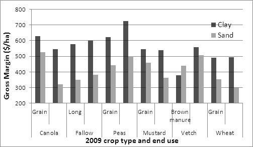
Figure 3. Sand and clay site mean three year gross margin $/ha with crop type and
end use grown in 2009 followed by Correll wheat in 2010 and 2011.
BCG have commenced research to investigate use of summer fallow rain and stored soil water to plant and establish wheat and canola crops much earlier than is currently practiced. Separate trials at the BCG main site this year are comparing different long season wheat and canola varieties planted in March and established on soil water alone (Figure 4). Given the very dry autumn of 2012 (a continuing climatic trend caused by reduced frequency of cut-off lows), these early sown crops now stand a much better chance of flowering on time and achieving good water-use efficiency compared to the majority of crops in the Wimmera and Mallee that did not emerge until June. These trials will be on display at the BCG field day on 13 September 2012.
For more information on these trials please see the BCG 2011, 2010 and 2009 Season Research Results booklets and BCG website.
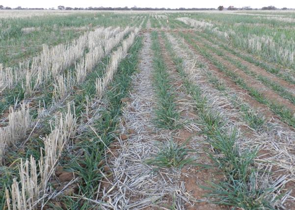
Figure 4. Winter wheat (EGA Wedgetail![]() ) sown in March 2012 at the BCG main site
) sown in March 2012 at the BCG main site
near Birchip (photo taken mid-June 2012). The plot on the right was mown in mid-May
2012 to simulate grazing.
Further reading
Kirkegaard JA, Hunt JR (2010) Increasing productivity by matching farming system management and genotype in water-limited environments. Journal of Experimental Botany 61 (15), 4129-4143.
Contact details
James Hunt
GPO Box 1600 Canberra ACT 2601
james.hunt@csiro.au
Was this page helpful?
YOUR FEEDBACK