How much water is lost from northern crop systems by soil evaporation

Do agronomic models accurately represent this loss?

GRDC code: ERM00002

Authors

Jenny Foley, Department of Natural Resources and Mines, Toowoomba, Qld.
Justin Fainges, CSIRO, Toowoomba, Qld.

Globally 20% of terrestrial rain is evaporated through soil, while 40% is transpired through plants (Oki et al. 2006, Or et al. 2013).  Studies from around the globe show that in agricultural cropping lands evaporative losses can be as high as 30 -75% of rain during a growing season (Mellouli et al. 2000). Grain growers in the Northern GRDC region, who are heavily reliant on rainfall and stored soil water to grow crops, are well aware of these significant losses and factor them accordingly into their decision making processes. This is often done with the aid of agronomic models, which are used to devise fallow management strategies, irrigation strategies, and in more complex simulation models to help growers decide how to use water efficiently. For researchers and funding bodies these same models are used to determine the size of the gap between potential and actual yield in agronomic research and to predict runoff, deep drainage, flow into rivers, and recharge to groundwater in landscape research.

Errors in modelling the soil evaporation component of the soil water balance can have a significant impact on the numbers produced. This in turn affects decision-making at all levels. Our local knowledge of soil evaporation for northern region soils and climates has until now been limited, with the implications for water balance modelling being a potentially significant under or over prediction of the other terms, including runoff and deep drainage. Given the importance of soil evaporation in influencing how much water will be stored during a fallow and its potential to vary with climate, soils and land management practices, it is timely (within the scope of this project) to assess the way in which we are accounting for these losses in our models

Most of our soil water balance and agronomic models (APSIM-SoilWat, HowLeaky, HowWet) use the two stage Ritchie model (Ritchie 1972) to describe soil evaporation. Stage 1 drying occurs after rain when the soil is wet and able to supply water fast enough to satisfy the evaporative demand (Figure 1). Evaporation occurs at the same rate as daily potential evaporation (PE), and lasts until a specified amount of evaporation is reached, t₁ (U, mm). Stage 2 drying then commences, once the limiting availability of water exerts a controlling influence on soil evaporation. This stage is time-dependent according a specified value called CONA (mm/day^0.5).  Selecting what U and CONA values to use is still largely an intuitive and experience based process. In many cases, without the availability of measured data, modellers simply use the given default values in the model.

Figure 1. The Richie model

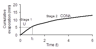
Figure 1 text description

The following are approximations:

• Stage 1 shows cumulative evaporation is up to 5mm, when Time is equal to 1.
• Stage 2 shows an increase with cumulative evaporation up to 15mm, when Time reaches 6.

Measuring soil evaporation

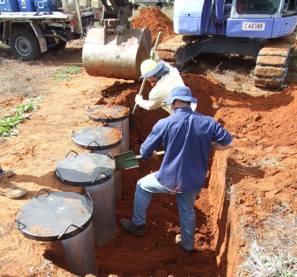
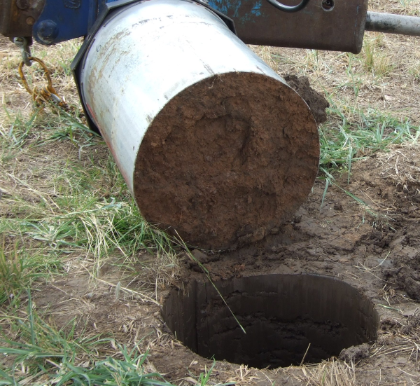
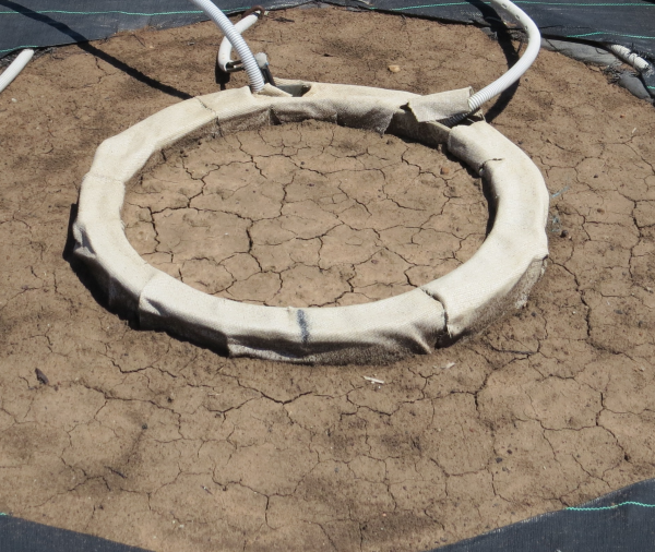
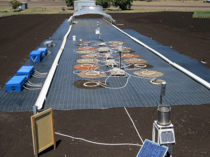
During 2009-10 we built a rather unique “Lysimeter Farm” at Kingsthorpe Research Station (20 km west of Toowoomba, Qld.) to enable us to measure soil evaporation directly. The farm houses 18 large cylindrical undisturbed soil monolith weighing lysimeters, 0.6 m diameter x 0.8 m deep (see Photo 1).  Each of these lysimeters sits upon a configuration of strain gauges within a liner buried 1 m in the soil. Weight gains from natural rainfall, or losses from evaporation, are recorded every 15 minutes. Four key soils of the northern growing region with clay contents ranging from 12-78% were cored for the lysimeter study; a Black Vertosol from the Darling Downs, two Grey Vertosols from Nindigully and Roma, and a Red Kandosol from St George. There are also water filled lysimeters at each end of the array for recording pan evaporation.

Between January 2010 and December 2013 we compiled a dataset for each soil of ~40 wetting-drying curves after rainfall events (> 4 mm) with a diversity of rainfalls i.e. light to heavy falls, climates and soil surface antecedent water contents. The duration of each drying curve varied from 3-78 days. A rainout shelter was used during selective rain events to extend drying curves. A spectrum of both wet (flux limited) and dry (supply limited) evaporative conditions are represented in this comprehensive dataset.

Figure 2. Lysimeter facility at Kingsthorpe Research Station, showing leachate collection setup (blue boxes left of image), 16 soil and 2 water lysimeters installed in the ground, a weather station, centrally positioned weatherproof boxes housing loggers and multiplexers, and a rainout shelter at the far end.

How much do our soils evaporate?

Rainfall amount in combination with antecedent soil water, i.e. amount of water available to evaporate, has a strong influence on evaporation rates. When rain falls on already wet soil, daily rates tend to be higher as soil evaporation is only flux limited. However when the soil is dry, small rainfall events result in small evaporation rates regardless of PE, i.e. soil evaporation is supply limited (see circled points in Figure 3).

The daily fallow evaporative loss averaged for all soils and years was ~0.75 mm per day. There were distinct seasonal differences in evaporation rates with around 0.6 mm per day lost during winter and 1 mm per day lost during summer.

Evaporation data (analysed using linear mixed models) with rainfalls grouped into small, medium and large falls, revealed complex interactions between soils, seasons, rainfall amount and duration of drying curves. For example – for large rainfall events (>30 mm), season and duration of the drying curve significantly influence daily evaporation, rather than soil type, i.e. evaporative demand and available water are the dominant drivers. However, for medium rainfall events (10-30 mm) daily evaporation is influenced by seasons and soil types.

Not all soils lose water at the same rate. The Black Vertosol has a significantly higher evaporative loss throughout the year than the others soils, loosing 40-50 mm per year more water than the other soils. All soils lose more water in the hotter months. This is not just due to seasonal variations in PE, but also due to the amount of rainfall, antecedent soil water and the way the different soils lose water when evaporative demand is higher or lower.

Figure 3. Cumulative soil evaporation for each drying curve showing a linear response to time.

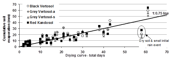
Figure 3 text description

The following are approximations:

Black Vertisol, Grey Vertisol-a, Grey Vertisol-s and Red Kandosol all recorded an increase in cumulative evapororation over 70 days, from 0mm to 55mm. At 60 days there was a decrease of 10-15mm (approximately) in cumulative evapororation due to dry soil and and a small initial rain event, with Black Vertisol at 20mm, Grey Vertisol-a at 20mm, Grey Vertisol-s at 15mm and Red Kandosol at 28mm.

Soils and seasonal variations in U and CONA

High evaporative losses due to Stage 1 drying were observed infrequently in the paddock under natural rainfall and climatic conditions. Typical weather in south east Queensland is slightly summer dominant rainfall, with frequent high intensity (usually late afternoon) thunderstorms followed by humid conditions and good infiltration into the soil profile overnight when evaporative demand is low. Throughout the year there are also frequent drizzly rainfalls with prolonged overcast, humid conditions and damp soil and atmosphere (reducing solar input and the evaporative gradient). These smaller drizzly falls frequently persist after a main rain event. This type of weather produces low atmospheric demand and low PE, suppressing initial evaporative losses. At the same time soil moisture redistribution from the top few cm to deeper in the soil profile continues. By the time atmospheric demand increases, soil water has become less available and evaporative drying had moved past first stage drying behaviour.

Across all drying curves, initial evaporative losses after rain were between 0.1-3 mm in the first 24 hr. After 48 hr 0.4-6 mm had evaporated from most curves with the majority <4 mm. A conservative estimate of 2 is recommended for U as a modelling parameter. This is lower than most values commonly in use (3-8), however in agreement with recommendations from Yunusa et al. (1994) for Australian conditions.

CONA values were calculated empirically from ~40 cumulative evaporation curves for each soil, and a summary is provided in Table 1. CONA was significantly higher for the Black Vertosol than other soils. Winter CONA values were significantly lower than the other seasons. The relationship between CONA and potential evaporation (PE) was also analysed and only a very weak positive relationship found.

Testing the Models – APSIM-SoilWat, APSIM-SWIM are they a good predictor of soil evaporation?

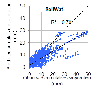
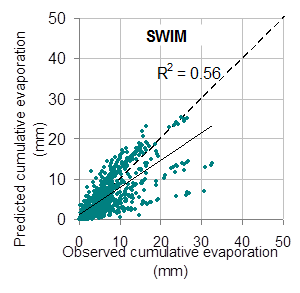
APSIM’s ability to simulate the evaporative process was tested using empirically derived U and CONA and the measured soil evaporation data. APSIM (Keating et al. 2003) contains two water balance models; SoilWat, a cascading bucket model based on the Ritchie model, and SWIM, a physical model of water movement based on a numerical solution of the Richards’ equation and the advection-dispersion equation. Drying periods were modelled separately in APSIM with each period being its own simulation. For the SoilWat model, our experimentally derived U and CONA values for each soil and summer/winter seasonal averages were used (Table 1). SWIM is a physical model so requires no parameters beyond those specified by the soil. Actual measured starting waters, soil hydraulic properties and climate data were used. The model was then run for the duration of the period and predicted cumulative evaporation of both models compared against observed data (Figure 4a,b).

Both models give a very similar response indicating that our empirically derived U and CONA values for SoilWat were accurate in describing the measured dataset. Both models show a propensity to under predict evaporation, especially during long drying periods. Kodur also found this when modelling this dataset with HowLeaky (Rattray et al. 2004), which uses SoilWat to model the soil water balance, but with only a single U and CONA value as evaporative inputs (Kodur et al. 2013). The under prediction is often linear (Figure 4a,b), indicating inaccurate initial conditions rather than a deficiency in either model is the cause.

The large difference in the number of simulations run for each model can be attributed to the physical nature of SWIM. SWIM requires a hydraulic gradient in order to move water between layers, so for soils that are at or above DUL this gradient is very low and SWIM can have difficulty finding a solution. In addition, SWIM was unable to find a solution for any Mulga View simulations due to the fact that it is a sandy soil and exceeded DUL by a significant amount at the start of every drying period.

Overall, both models are acceptable for modelling soil evaporation over a range of soils and seasons provided accurate soil physical properties and starting water states are known.

Figure 4. Predicted and observed plot for cumulative soil evaporation using a) SoilWat, and b) SWIM.

References

Keating BA, Carberry PS, Hammer GL, Probert ME, Robertson MJ, Holzworth D, Huth NI, Hargreaves JNG, Meinke H, Hochman Z, McLean G, Verburg K, Snow V, Dimes JP, Silburn M, Wang E, Brown S, Bristow KL, Asseng S, Chapman S, McCown RL, Freebairn DM, Smith CJ (2003) An overview of APSIM, a model designed for farming systems simulation.  European Journal of Agronomy 18, 267-288.

Kodur S, Foley JL, Silburn DM, Waters D (2013)  Evaluation of modelled and measured evaporation from a bare Vertosol soil in south east Queensland, Australia. MODSIM-2013 20^th International Congress on Modelling and Simulation, 1-6 December 2013, Adelaide, Australia.

Mellouli HJ, van Wesemael B, Poesen J, Hartmann R (2000) Evaporation losses from bare soils as influenced by cultivation techniques in semi-arid regions. Agricultural Water Management 42:355–369.

Oki T, Kanae S (2006) Global hydrological cycles and world water resources. Science 313:1068–1072.

Or D, Lehmann P, Shahraeeni E, Shokri N (2013) Advances in Soil Evaporation Physics—A Review. Vadose Zone Journal 12(4).

Rattray DJ, Freebairn DM, McClymont D, Silburn DM, Owens J, Robinson B (2004)  HOWLEAKY? The journey to demystifying ‘simple’ technology.  Paper 422. In ISCO 2004 ‘Conserving Soil and Water for Society: Sharing Solutions’, 13th International Soil Conservation Organisation Conference, Brisbane, July 2004. (Eds SR Raine, AJW Biggs, NW Menzies, DM Freebairn, PE Tolmie) (ASSSI/IECA: Brisbane.

Ritchie JT (1972) A model for predicting evaporation from a row crop with incomplete cover. Water Resources Research 8:1204–1213.

Yunusa IAM, Sedgley RH, Tennant D (1994) Evaporation from bare soil in south-western Australia - a test of two models using lysimetry. Australian Journal of Soil Research 32(3):437–446.

Contact details

Jenny Foley
Department of Natural Resources and Mines
Ph: 07 45291270
Mb: 0428309323
Email: jenny.foley@dnrm.qld.gov.au

Reviewed by

Dr Mark Silburn, Department of Natural Resources and Mines, Toowoomba, Qld.