Global and commercial realities facing Australian grain growers
Author: Mick Keogh | Date: 06 Feb 2013
Mick Keogh
Australian Farm Institute
Take Home Messages:
- Grain growers in Australia operate in a unique business environment, fully exposed to the volatility of international grain markets, and also more exposed to the vagaries of the Australian climate than perhaps any other businesses.
- Changes internationally and within Australia over the past decade are likely to mean that the strategies grain growers have previously used to manage some of the risks they face are no longer adequate, and may need changing in order for their business to remain profitable in the future.
The past decade
The operating environment for managers of Australian grain growing businesses has changed markedly over the past decade as a consequence of developments that have occurred internationally, as well as within Australia. While each of the changes has been discussed in detail over the years, there is value in listing all of them because it is their combined effects that have to be considered by grain growers, not their impacts in isolation.
Major changes that have occurred in global grain and oilseed markets over the past decade include the following:
- Government policies, in particular in the EU and the USA, have been adjusted so that they no longer encourage excess production, and governments in both these locations no longer hold large stocks of grain or oilseeds, as they did in the past, that were used to intervene in grain markets at different times.
- Government-mandated renewable fuel policies in major grain producing nations such as the USA and Brazil, and in the EU, have created a major new and largely inelastic source of demand for grains and oilseeds, which some now estimate to amount to 10% of global grain and oilseed production, and which have accounted for up to 40% of US corn production in specific years.
- Middle class consumers in developing nations have increased the proportion of animal protein in their diets which, in combination with growth in the populations of these nations has dramatically increased the demand for grains and oilseeds suitable for use as stockfeed.
- The global grain trading sector has experienced a period of major consolidation over the past decade, which has led to international grain and oilseed markets being dominated by six major corporations – Archer Daniels Midlands (ADM), Bunge, Cargill, Louis Dreyfus, Glencore and Marubeni. These six multinational grain traders are estimated to account for in excess of 75% of all trade grain and oilseeds globally, and that consolidation is continuing, as recent events in Australia highlight.
- The emergence of developing nation grain exporters, such as the nations of eastern Europe as well as Brazil and Argentina, has added a new dimension to global grain markets with a number of these suppliers having interventionist governments, the actions of which have at different times created great uncertainty and volatility in international grain markets.
- The growth of speculative interest in soft-commodity derivative markets such as futures and options has resulted in changes in these markets as speculator participants begin to outnumber participants holding physical stocks. This is leading these markets to behave in ways that are not necessary consistent with supply and demand fundamentals, especially around close-out dates for contracts.
Some major changes have also occurred within the Australian economy and the domestic grain market. These include:
- The deregulation of the Australian grain and oilseeds markets. The result being that with the exception of the rice industry, there is no statutory marketing or generic promotion occurring within the Australian grain and oilseeds industries.
- Technological changes have resulted in increased mechanization. The ever-growing use of computer and GPS-enhanced equipment, and continuing increases in the area of crops that can be planted and harvested per person.
- The mining boom has created very strong demand for labor in many parts of regional Australia, and has also resulted in labour cost escalation even in areas where there is not a strong mining presence.
- For extended periods during the last decade, seasonal rainfall across much of the grain-growing areas of southern Australia was well below average, resulting in substantial reductions in national grain and oilseed output.
- There has been a significant change in the input supply and advisory sub-sectors servicing the industry, with an increase in the use of commercially-owned crop varieties (including GM crops) and a progressive reduction in the capacity of, and services available from, the public sector research, development and extension agencies – in particular State government agencies.
- The nature of government support for farm businesses in Australia has changed, with the Australian government announcing during 2012 that drought support measures would no longer include interest rate subsidies for those farm businesses judged to be viable in the long term but unable to meet their financial commitments due to exceptional drought.
- Finally, the persistently high value of the Australian dollar has meant that Australian grain prices are lower than they would otherwise have been, given historical exchange rates. This has brought some advantages in terms of relatively lower input and machinery costs, but on balance has meant Australian grain growers are at a disadvantage relative to the situation they would face under a lower $AUD exchange rate.
As noted earlier, each of these changes in isolation may have only limited impact on individual grain businesses, but in combination they all result in a significant change in the business environment in which grain farms operate.
Individual grain businesses will have been impacted in different ways by all these changes, depending on whether they are involved in grain or oilseed production, whether their production supplies human consumption or the energy or stock-feed market, and whether their principal markets are domestic or international.
One general conclusion that emerges from almost every analysis of the impact of these changes is that the result has been an increase in the volatility of global and domestic grain markets, which means that the level of risk has increased for these businesses, relative to what has been the case in the past.
This in turn dictates that for grain growing businesses to remain profitable in this more volatile and risky environment, grain growers will need to become better business managers.
Risk management
Risk management has always been an important aspect of operating successful farm businesses, and in broader national policy settings associated with agriculture, both in Australia and internationally. Throughout history, most government interventions in agricultural markets can be characterised as attempting to manage risk – either at the individual farm business level, or at a national level due to concerns about issues such as food security. Two of the largest existing agricultural policy programs (The Farm Bill in the USA and the Common Agricultural Policy in the EU) essentially involve policy measures to reduce farm business risks, and virtually every nation globally has some policy measures aimed at reducing or managing risks for agricultural businesses.
All business enterprises carry with them a range of risks, but the main focus of risk management analyses and policies relevant to agriculture have been on;
(a) production risk; which arises from the uncertainty associated with crop and livestock growth, as weather, disease, pests, and other factors affect both the quantity and quality of commodities produced, and
(b) price or market risk; which arises from uncertainty about the prices producers will receive for commodities and the cost of their inputs.
There are large numbers of research reports that analyse the nature of risks faced by agricultural businesses, and the success or otherwise of policies that aim to reduce or mitigate these risks[1]. In more recent times in Australia, these have included research which aimed to disaggregate the various elements of risk faced by grain producers in Western Australia (Kingwell, 2011), and research which aimed to evaluate different strategies (including the production of multiple commodities) available to farm business managers to manage risk (Hutchins and Nordblom, 2011)
Data and methodology
The objective of the analysis reported here is to gain a better understanding of the business volatility experienced by Australian farm managers, and to consider whether there may be options available that could assist them to better understand and manage volatility in their businesses. Volatility refers to the degree of variability of a particular measure or statistic over time, and is defined as a directionless measure of variation. (Gilbert and Morgan 2010).
Volatility can be quantified by calculating the extent to which an actual measured statistic diverts from the value that might be anticipated, assuming a smooth long-term trend. In a sense, volatility refers to the ‘unexpected’ or ‘unanticipated’ changes experienced by a farm business. While, in the case of a farm business, both revenue and costs can vary, the main focus in this analysis will be on revenue volatility, because to a large extent farm costs are driven by management decisions (such as how much crop will be sown or livestock produced) that are made based on revenue expectations, and therefore the revenue side of a farm business is the critical one from a profitability perspective.
Volatility is generally estimated by calculating the standard deviation of the percent difference between actual and trend value of a particular statistic over time (Productivity Commission, 2005). Trend values can be estimated in a number of ways, ranging from a simple linear best fit trend line to more complex mathematical methodologies. The appropriate methodology that should be utilised to generate longer-term trend lines is a topic of considerable debate amongst statisticians. However, in comparisons of relative volatility, such as are reported here, consistency in the methodology utilised to generate trend lines is more important than the actual methodology itself.
Given the variable and obviously non-linear nature of much of the commodity price and production data used in this analysis, it was determined that a third order polynomial trend line estimated using least squares analysis generally provided a reasonable trend estimate, and this same methodology was used as the basis for calculating all the volatility estimates.
Relative volatility of annual Australian agricultural output
A useful starting point in analysing volatility in Australian agriculture is to compare the volatility of measures of agricultural output in Australia with those of other nations. Annual agriculture output data compiled by the Food and Agriculture Organisation of the United Nations (FAO, 2011) over the period from 1961 to 2009 was utilised to develop trend output estimates for a selection of important agricultural nations, covering a range of developed and developing nations, and for which data was available. The standard deviation of the percentage variation between trend and actual output was then calculated. The results for each nation were indexed around the average, with the average set at an index value of 100. The results are shown in Table 1, based on the annual agricultural output value (constant 2004-2006 $US) and indexed volume of annual output for each nation.
Table 1. Index of volatility of national annual agricultural output by value and volume, 1961-2009. (Average volatility for 15 nations = 100). Data sourced from FAO, 2011.
| Country | Value of output | Indexed volume of output | ||||
|---|---|---|---|---|---|---|
| Agriculture | Crops | Livestock | Agriculture | Crops | Livestock | |
| Argentina | 135 | 123 | 151 | 115 | 107 | 138 |
| Australia | 186 | 204 | 91 | 143 | 173 | 119 |
| Brazil | 73 | 69 | 67 | 87 | 86 | 63 |
| Canada | 86 | 122 | 124 | 103 | 125 | 80 |
| Chile | 82 | 60 | 103 | 127 | 81 | 178 |
| Denmark | 43 | 90 | 124 | 63 | 98 | 57 |
| France | 74 | 77 | 32 | 73 | 76 | 51 |
| India | 89 | 66 | 38 | 69 | 56 | 45 |
| Mexico | 72 | 55 | 35 | 82 | 61 | 131 |
| Netherlands | 123 | 91 | 154 | 102 | 81 | 131 |
| New Zealand | 76 | 80 | 93 | 74 | 114 | 75 |
| Poland | 102 | 110 | 146 | 113 | 104 | 123 |
| South Africa | 98 | 111 | 100 | 110 | 132 | 94 |
| USA | 65 | 67 | 128 | 77 | 90 | 43 |
| Uruguay | 201 | 152 | 57 | 162 | 116 | 172 |
The data identifies that the volatility in the average value of Australian agricultural output has been the second highest of any of the nations included in the research over the forty year period for which data is available, and has been 86% higher than the average for all the nations included. When disaggregated into crops and livestock products, the data shows that the volatility of Australian crop production has been higher than for any other nation (either by value or by volume) over the period, and was more than 100% higher than the average for all other nations. In contrast, the volatility of Australian livestock production has been close to or below the average of all other nations over the same period.
These results assist in putting the issue of risk in perspective for Australian farm business managers. They highlight that, by international agricultural standards, Australian farm businesses have faced a more volatile operating environment than has been the case for farmers in almost all other nations over the last forty years.
Relative volatility of Australian economic sectors
Australian farm businesses compete with businesses in other sectors of the Australian economy for capital, human and natural resources. Therefore it is useful to consider the volatility of the agriculture sector relative to those other sectors of the economy, and also to identify whether the relative volatility of the agriculture sector has changed over time.
In order to compare the relative volatility of different sectors of the Australian economy, annual industry gross value added statistics, compiled by the Australian Bureau of Statics (ABS 2011) for the period from 1975 to 2011, were obtained for seventeen sectors of the Australian economy. Trend estimates were derived for annual industry output for each sector, and the percentage variability of actual industry output relative to trend was then calculated, in the same manner as described above. The results were calculated for the entire thirty-seven years for which data was available, and also on a decade-by-decade basis in order to obtain some perspective of relative changes in volatility for each industry sector over time. The results of this analysis are shown in Table 2.
Table 2. Index of relative volatility in annual value of output for major Australian economic sectors. Data sourced from ABS, 2011.
| Industry sector | Whole period 1975-2011 | 1975-84 | 1985-94 | 1995-04 | 2004-11 |
|---|---|---|---|---|---|
| Health care | 46 | 56 | 48 | 34 | 29 |
| Electricity, gas and waste | 47 | 59 | 35 | 31 | 60 |
| Public administration | 49 | 53 | 51 | 50 | 45 |
| Education and training | 54 | 75 | 43 | 27 | 42 |
| Transport | 72 | 90 | 72 | 45 | 83 |
| Rental and real estate services | 73 | 64 | 88 | 77 | 102 |
| Manufacturing | 75 | 79 | 91 | 63 | 76 |
| Retail trade | 75 | 62 | 95 | 59 | 107 |
| Professional services | 97 | 67 | 132 | 116 | 83 |
| Accommodation and food services | 103 | 85 | 118 | 112 | 150 |
| Administrative services | 115 | 122 | 104 | 161 | 111 |
| Wholesale trade | 120 | 106 | 172 | 76 | 65 |
| IT, Media and telecommunications | 120 | 167 | 53 | 64 | 65 |
| Mining | 128 | 159 | 108 | 124 | 122 |
| Construction | 134 | 94 | 162 | 200 | 116 |
| Finance and insurance | 157 | 106 | 208 | 87 | 153 |
| Agriculture | 234 | 257 | 120 | 374 | 293 |
| All industry average | 100 | 100 | 100 | 100 | 100 |
The results in the table indicate that the agriculture industry has been, and remains the most volatile sector of the Australian economy over the past four decades, and that the value of output from the agriculture sector has been almost two and a half times more volatile than the average for all the major sectors the economy.
The above results also indicate that the agriculture sector may have become relatively more volatile over the most recent two decades, a result that is not surprising given factors discussed earlier.
Relative volatility of Australian agricultural commodity sub-sectors
Within the Australian farm sector, there are a range of different commodity sub-sectors, each of which experiences differing levels of volatility in both commodity prices and production volumes. The volatility of the total annual value of production of a specific commodity is a combination of both seasonal conditions (affecting production intentions, crop yields and livestock growth rates) and commodity prices (affecting production intentions and revenue), with commodity prices affected by a range of domestic and international market factors, depending on the commodity involved. Volatility of production also varies depending on regional location, with some regions being ‘safer’ and some less so in terms of seasonal rainfall and temperature expectations.
To compare volatility between commodity sub-sectors, the annual value of output from each of the main commodity sub-sectors was obtained for the period from 1961 through to 2009. Trend estimates were calculated for each commodity, and the volatility of each was then calculated using the same methodology as outlined above. The relative volatility of each commodity sub-sector was then indexed for the entire period, and for each of the decades over the period under examination.
Table 3. Index of relative volatility in annual value of output for major Australian agricultural commodity sub-sectors. Data sourced from FAO and ABS.
| Commodity sub-sector | Whole period | 1961-70 | 1971-80 | 1981-90 | 1991-00 | 2001-09 |
|---|---|---|---|---|---|---|
| Fruit and nuts | 57 | 61 | 66 | 32 | 40 | 79 |
| Vegetables | 62 | 91 | 64 | 67 | 41 | 56 |
| Grains and oilseeds | 195 | 190 | 149 | 303 | 255 | 286 |
| Dairy | 103 | 107 | 90 | 40 | 113 | 130 |
| Beef | 128 | 119 | 164 | 94 | 58 | 51 |
| Sheepmeats | 108 | 68 | 181 | 87 | 56 | 101 |
| Pork | 78 | 69 | 123 | 43 | 29 | 73 |
| Poultry | 60 | 111 | 31 | 32 | 50 | 27 |
| Wool | 101 | 82 | 87 | 216 | 131 | 84 |
| Sugar | 109 | 103 | 45 | 86 | 227 | 112 |
| All commodity average | 100 | 100 | 100 | 100 | 100 | 100 |
Some of the above results are expected given developments that have occurred in each of the commodity sub-sectors over the period in question. The beef industry, for example, experienced a very turbulent period during the 1970’s when cattle prices slumped and became virtually worthless, resulting in an exodus from the industry. The wool industry also experienced considerable turmoil during the late 1980s and early 1990s as sheep numbers increased dramatically due to high prices in the second half of the 1980s, and then declined due to the price crash associated with the cessation of the reserve price scheme in early 1991.
While recognising that these effects distort results for specific commodities, there are a number of generalizations that can be made arising from the results displayed in this table. Firstly, the horticulture sub-sectors have experienced considerably less volatility than the broadacre sub-sectors such as grains, beef and sheepmeats. This is to be anticipated as fruit and vegetable production normally occurs under irrigation, therefore reducing production variation due to seasonal conditions. Fruit and nut production also involves a relatively fixed stock of trees that cannot quickly be adjusted given changes in commodity prices. As would also be expected, the intensive livestock sub-sectors (pork and poultry) have also experienced considerably less volatility than the broadacre sub-sectors, again because these sub-sectors are largely unaffected by seasonal conditions.
What is also quite evident is that the grains and oilseed sub-sectors have consistently experienced a much higher level of volatility than any other sub-sector of agriculture. This is as expected given that non-irrigated grains and oilseed production in particular can be greatly affected by adverse seasonal conditions such as low or untimely rainfall. Grain and oilseed production also involves annual decisions by farmers about crop varieties and areas, which means farmers can respond quickly depending on prevailing prices and seasonal conditions. Broadacre livestock production, on the other hand, generally involves longer-term decision-making, and livestock are often retained for some time despite poor seasonal conditions, and can be maintained during droughts by utilising supplementary feed.
The extent to which volatility in a particular commodity sub-sector is a consequence of decisions by farmers, or is an intrinsic feature of the production system and associated markets is difficult to determine. Recent research by Kingwell (Kingwell, 2011) addressed this question in an analysis of the volatility of wheat revenue for Australian farmers over the last fifteen years. That analysis separated out the various components of revenue variance for wheat production (price volatility, wheat area planted and wheat yields) and concluded that the de-trended volatility of wheat revenue has more than doubled in every main wheat-growing state of Australia over the last fifteen years. That research identified changes in the area of wheat sown (a management decision made by farmers in response to prevailing seasons and prices) was mostly a minor source of revenue variance. It was found that the major sources of revenue volatility were yield variance (associated with seasonal conditions) and that while less important, price changes also increased in importance as a source of revenue volatility over the period in question.
The data displayed in Table 3 appears to confirm these findings, with the volatility of the total value of production of the “Grains and Oilseeds” sub-sector increasing substantially over recent decades, especially relative to other commodity sub-sectors.
Relative volatility of Australian agricultural commodity prices
As noted above, the volatility of agricultural commodity prices is likely to be an important component of the overall revenue volatility experienced by Australian farm businesses. The volatility of global agricultural commodity prices has been the subject of a number of research studies over recent years (Gilbert and Morgan 2010, Winsen et. al. 2011, Poon and Weersink 2011, Kimura and Anton 2011, Kimura, Anton and LeThi 2010, FAO et. al. 2011, High Level Panel of Experts 2011). Many of these analyses conclude that agricultural commodity prices have been more volatile over recent years than they were during the 1990s and early 2000s, but not more volatile that they were during the 1970s.
Any examination of the volatility of agricultural commodity prices experienced by Australian farmers is complicated by the fact that there is a lack of consistent, long term commodity price series that can be utilised for such analyses. This applies in particular for horticultural products and some crops. Further, some of the available long-term price series provide averaged annual commodity price data, which can tend to smooth commodity price volatility relative to what is experienced by the manager of a farm business. As recent years have highlighted, there can be considerable price variation within a year around the annual average. Long-term (1980 to present) monthly agricultural commodity price data series for a number of Australian agricultural commodities are maintained by the International Monetary Fund (IMF 2011), although these are generally the prices prevailing at port of destination rather than Australian farmgate prices.
There are a limited number of longer-term monthly price series data available for wool, beef and wheat which can be used to analyse whether price volatility has changed over recent years, although even these have limitations in that some of the data is sourced internationally. Table 4 provides details of available data sources, and a necessarily limited analysis of changes in commodity price volatility over recent decades.
Table 4. Index of relative volatility of prices for major Australian agricultural commodities.
| Commodity | Price series | Source | Between commodities | Within commodities over time | |||
|---|---|---|---|---|---|---|---|
| 1980-2011 | 1980-1989 | 1990-1999 | 2000-2011 | Average | |||
| Beef (export) | Average monthly export price $AUD, (1983-2011) | Westpac and MLA | 82 | 86 | 132 | 82 | 100 |
| Beef (domestic) | Eastern Young Cattle Indicator (EYCI) monthly, (1996-2011) | MLA | 74 | 119 | 81 | 100 | |
| Wheat | US No.1 Hard Red Wheat FOB USA. Monthly, (1980-2011) | IMF | 117 | 57 | 110 | 133 | 100 |
| Wool | Eastern Market Indicator. Monthly average (1992-2011) | AWEX | 126 | 103 | 97 | 100 | |
| Average | 100 | ||||||
Unfortunately, data limitations make the results less than conclusive, and the lack of data series extending back to the 1970's means it is not possible to compare current price volatility levels with those prevailing prior to the 1980's. The main conclusions from these results are that wheat and wool prices appear to be more volatile than beef prices; that beef and wool prices appear to have become less volatile in the most recent decade; and that wheat prices appear to have become more volatile over the most recent decades.
Analysis of the price volatility of different agricultural commodities also provides an opportunity to examine the extent to which movements of prices around long-term trends follow similar or different patterns. If the variations in commodity prices for different commodities follow similar trends, then enterprise diversification may not provide an opportunity to reduce farm business risk. Alternatively, if commodity price variations follow independent trends, enterprise diversification may provide opportunities to reduce business risks.
Figure 1 displays the percentage variation of actual commodity prices from long-term trends for three major Australian broadacre farm commodities. The graph indicates that generally, price variations for the three commodities tend to follow independent patterns, although it also highlights that there have been some periods (for example 1997-2000) where prices for all three commodities were lower than prevailing longer-term trends.
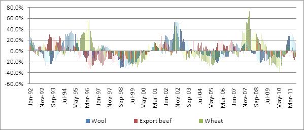
Figure 1. Percentage variation of the prices of three major broadacre commodities from their long-term trend price levels.
If commodity prices were the sole driver of farm revenue volatility, then it appears that enterprise diversification should provide farm business managers with a means of reducing farm business risk. However, as noted earlier it is the combination of seasonal and commodity price factors that determines broadacre farm revenue, therefore analysing commodity price trends in isolation does not provide a complete picture.
Management of volatility at the farm level
A high level of volatility in isolation does not necessarily present a challenge for managers of farm businesses. For example, volatile but relatively high commodity prices can provide an opportunity for profitable farm operations given the availability of suitable risk management options or a strong farm balance sheet which enables ready access to finance. Generally however, higher volatility presents greater management challenges for farm businesses because of the narrow operating margin of most farms, the fixed nature of farm assets, and the limitations presented by climate and natural resources such as land and water.
Farm survey data collected by ABARES over the past twenty year period provides an opportunity to examine how well Australian broadacre farmers have managed the volatile business environment in which they have been operating. ABARES surveys a structured sample of Australian broadacre farm businesses each year, obtaining both financial and production data. The resulting data is made available on the online ABARES Agsurf database, and is able to be disaggregated in a number of different ways. By examining changes in farm capital values, farm profits and farm debt levels over the period, some sense may be obtained of how well farm business managers are managing risks that are inherent in the volatile business environment in which they operate.
Data obtained from ABARES annual farm surveys over the period from 1990 to 2011 was used to examine in particular changes that have occurred in farm income and debt levels for crop farms and mixed livestock and crop farms. Because the data is subject to annual variation depending on commodity prices and seasons, a clearer picture of changes that have occurred can be obtained by comparing data averaged over a five year period. For this analysis, data averaged over two five year periods was used for the comparison (1990-94 and 2007-11). All values were expressed in 2010-11 dollars. The available data was disaggregated on the basis of commodity production (an all farm average, enterprises producing mainly crops, and mixed livestock and crop enterprises), on the scale of the farm (determined by gross turnover), and on the State in which farms were located. In each case, averages for the 1900-1994 period were compared with averages for the 2007-2011 period to obtain a clear perspective of changes that have occurred in those businesses over time. The results of the analysis are displayed in Table 5.
Table 5. Real changes in farm financial characteristics, by farm turnover category.
| Value of land and fixed improvement ($) | Farm business debt at 30 June ($) (1) | Total crop gross receipts ($) | Total cash receipts ($) | Farm cash income ($) | ||
|---|---|---|---|---|---|---|
| Farm/size location | Enterprise |
Percent change from 1990–94 to 2007-11 |
||||
|
Australia |
Allindustries | 162% | 135% | 77% | 45% | 36% |
| Crop | 237% | 229% | 64% | 65% | 34% | |
| Mixed livestock | 165% | 102% | 23% | 24% | 10% | |
| Sheep | 98% | 47% | 227% | 29% | 96% | |
| Beef | 148% | 139% | 51% | 32% | 3% | |
| Sheep/Beef | 164% | 99% | 157% | 49% | 82% | |
|
Less than $100,000 |
All industries | 84% | 9% | -52% | -26% | -80% |
| Crop | 58% | 41% | -56% | -35% | -176% | |
| Mixedlivestock | 128% | 16% | -62% | -32% | -132% | |
| Sheep | 62% | -17% | -75% | -26% | -60% | |
| Beef | 72% | 31% | -64% | -26% | -48% | |
| Sheep/Beef | 89% | 23% | -63% | -1% | 9% | |
|
$100,000-$200,000 |
All industries | 78% | -3% | -51% | -33% | -62% |
| Crop | 125% | 53% | -44% | -32% | -112% | |
| Mixedlivestock | 97% | 10% | -53% | -31% | -77% | |
| Sheep | 40% | -32% | -29% | -34% | -1% | |
| Beef | 61% | 3% | -52% | -36% | -47% | |
| Sheep/Beef | 58% | -31% | -70% | -31% | -35% | |
|
$200,000-$400,000 |
All industries | 93% | 7% | -50% | -33% | -43% |
| Crop | 95% | 34% | -38% | -33% | -68% | |
| Mixedlivestock | 112% | 9% | -47% | -31% | -49% | |
| Sheep | 29% | -23% | 4% | -31% | -4% | |
| Beef | 99% | 2% | -80% | -38% | -38% | |
| Sheep/Beef | 59% | -16% | -10% | -31% | -17% | |
|
> than $400,000 |
All industries | 108% | 86% | 23% | 1% | 0% |
| Crop | 187% | 134% | 19% | 23% | 19% | |
| Mixedlivestock | 90% | 66% | 0% | -7% | -4% | |
| Sheep | 26% | 21% | 102% | -15% | 33% | |
| Beef | 129% | 77% | 235% | -13% | -33% | |
| Sheep/Beef | 56% | 24% | 74% | -15% | -1% | |
Table 6. Real changes in farm financial characteristics, by location.
Real changes in farm financial characteristics, by location.
| Value of land and fixed improvements ($) | Farm business debt at 30 June ($) (1) | Total crop gross receipts ($) | Total cash receipts ($) | Farm cash income ($) | ||
|---|---|---|---|---|---|---|
|
New South Wales |
All industries | 126% | 125% | 51% | 28% | -13% |
| Crop | 231% | 224% | 24% | 35% | -32% | |
| Mixed livestock | 130% | 95% | -15% | 4% | -42% | |
| Sheep | 91% | 85% | 204% | 36% | 76% | |
| Beef | 104% | 110% | 212% | 31% | -22% | |
| Sheep/Beef | 106% | 62% | 63% | 15% | 17% | |
|
Victoria |
All industries | 140% | 104% | 99% | 53% | 92% |
| Crop | 176% | 215% | 46% | 50% | 42% | |
| Mixed livestock | 227% | 106% | 51% | 56% | 3% | |
| Sheep | 101% | 17% | 54% | 36% | 121% | |
| Beef | 75% | 79% | 4% | 10% | 26% | |
| Sheep/Beef | 269% | 177% | 218% | 152% | 314% | |
|
Queensland |
All industries | 175% | 116% | 25% | 31% | 20% |
| Crop | 194% | 170% | 107% | 97% | 116% | |
| Mixed livestock | 150% | 100% | 9% | 17% | -4% | |
| Sheep | 120% | -25% | 162% | -21% | 116% | |
| Beef | 160% | 143% | -24% | 28% | -4% | |
| Sheep/Beef | 172% | 61% | 163% | 9% | 77% | |
|
South Australia |
All industries | 150% | 99% | 73% | 55% | 62% |
| Crop | 197% | 135% | 66% | 55% | 46% | |
| Mixed livestock | 121% | 77% | 36% | 45% | 38% | |
| Sheep | 77% | 12% | 134% | 19% | 132% | |
| Beef | 120% | 150% | 110% | 16% | -55% | |
| Sheep/Beef | 259% | 160% | 208% | 116% | 244% | |
|
Western Australia |
All industries | 271% | 231% | 125% | 73% | 72% |
| Crop | 404% | 344% | 101% | 98% | 72% | |
| Mixed livestock | 212% | 132% | 70% | 38% | 57% | |
| Sheep | 163% | 133% | 459% | 38% | 56% | |
| Beef | 401% | 341% | 1139% | 105% | 114% | |
| Sheep/Beef | 216% | 235% | 1225% | 74% | -3% | |
|
Tasmania |
All industries | 104% | 78% | 103% | 17% | 39% |
| Sheep | 61% | 30% | 62% | 25% | 75% | |
| Beef | 169% | 88% | 202% | -12% | -23% | |
| Sheep/Beef | 128% | 148% | 128% | 55% | 146% | |
| Northern Territory | All industries | 478% | 97% | -22% | 100% | 272% |
Based on the results displayed in the above tables, average farm business debt levels for all broadacre farms increased by an average factor of 135%, but for specialist crop farms, the increase in average debt levels was 229%, almost double the national average. In comparison, mixed livestock and crop farms recorded an increase of 102% in average farm debt levels.
This significant increase in farm debt levels coincided with a much more modest increase in cash receipts (which include drought support payments), and relatively small changes in net farm cash income for the average Australian broadacre farm businesses. (Net farm cash income is calculated by deducting total farm cash costs from total farm cash receipts. Farm cash costs exclude debt repayment or owner/operator wages) The relatively small change in net farm cash incomes compared to change in total receipts is likely a result of input cost increases over the period, including interests costs associated with higher debt levels.
The data highlights that for mid-sized farms (that is, those with between $100,000 and $400,000 in annual turnover), the farm business debt levels of crop farms increased by more than that of similar-sized mixed livestock and crop farms over the period, but at the same time net farm cash income levels of crop farms declined by more than that of the mixed livestock crop farms, and more than the average for all farms. It is only in the case of the largest sized crop farms (those with turnover in excess of $400,000 per annum) that the change in net farm cash income was greater than that of the mixed livestock and crop farms. These results indicate that on average, mid-sized cropping businesses now appear to have much less capacity to manage volatility than was the case during the early 1990s.
At the State level, it is apparent that on-average, farm businesses in New South Wales experienced a reduction in real annual farm cash income over the period, although it needs to be remembered that there are a greater proportion of smaller farms in NSW than in states such as Western Australia (and these farms may include lifestyle farms that are not run to generate a profit) which may negatively affect state averages, and also that drought conditions were generally considered to be worse in eastern Australia than Western Australia over the period. Farm businesses in Victoria, Western Australia, and the Northern Territory experienced strong growth in farm cash income over the period, while farm businesses in Queensland, South Australia and Tasmania experienced more modest growth.
Debt levels of farm businesses involved in cropping generally grew more than the debt levels of farm businesses involved in other enterprises, especially in New South Wales, Victoria, Queensland and Western Australia. In most cases these increased debt levels coincided with large increases in the value of land and fixed improvements of these farm businesses, indicating that the increased debt may be associated with an expansion of the scale of the business.
In isolation, the increases in farm debt levels shown in the above Tables indicate that Australian broadacre farm businesses are now likely to be less able to manage business volatility than was the case during the 1990s, whilst at the same time evidence indicates that the business environment for these enterprises has become more volatile, and that applies in particular for grains and oilseed enterprises. The increase in debt levels has been accompanied in some instances by increases in gross farm revenue, which should have improved the capacity of farm businesses to manage additional debt, although increased costs (including interest costs) has meant that increases in net farm income have been much more modest.
A key indicator often used to judge whether or not a business will be able to manage debt is the equity ratio of the business. It would be anticipated that, given higher debt levels, this ratio would have declined over the last two decades. However, the ABARES survey data indicates that this is not the case, and that equity ratios have been relatively stable over the period in question, albeit with some reduction in equity ratios for crop specialists relative to all farms and mixed livestock crop farms.
Part of the reason for the relatively stable equity ratios is that there have been large increases recorded in the average value of land and fixed improvements for farms over the period, especially in the case of crop specialists, as can also be observed from the above table.
A critical question is whether these increases in the value of farm capital assets are as a consequence of increases in land values, or due to an expansion in the average area of land owned by the farm business. If the increases in capital values are largely a result of increases in land values, then observed equity ratios may not be a reliable gauge of the ability of the farm business to service increased debt, and ultimately to manage volatility. The data displayed in Table 6 provides some information to assist in answering this question.
It shows that average farm land areas have increased by 14% over the period, but in the case of crop farms the average increase in land area over the two decades was almost 80%. The greatest increases in average farm land areas appear to have occurred in NSW and Western Australia, and for farms with more than $400,000 in annual turnover. The data displayed in Table 6 also highlights that the average area cropped per farm per annum has increased by substantially more than the increase in average farm area, indicating that cropping intensity (the proportion of total farm area sown to crop) has increased over the period, and that on mixed enterprise farms, cropping enterprises have become more important over the period under examination.
The fact that the percentage increase in farm land area has been less than the increase in the value of farm capital assets does indicate that at least a significant component of the increase in farm capital asset values may have been due to increases in average land values per hectare, and not just due to increases in average farm land area. This is confirmed by data available from a number of sources which shows that average farm land values per hectare increased quite rapidly in Australia in the years after 2001, which was a year of strong financial returns for many broadacre farm businesses in Australia. This has implications in that the increases in farm land values has provided an opportunity for farm businesses to increase debt while retaining equity levels, but may not mean that cash-flows to service that debt have also increased.
Table 7. Changes in farm areas, 1990 to 2010.
| Area operated (Hectares) | Area cropped (Hectares) | ||
|---|---|---|---|
| Farm size/ Location | Enterprise | Percent change from 1990-94 to 2006-10 | |
| Australia | All farms | 14% | 82% |
| Crop farms | 79% | 85% | |
| Mixed livestock/crops | 27% | 29% | |
| < $100,000 | All farms | 39% | 4% |
| Crop farms | -4% | 10% | |
| Mixed livestock/crops | 8% | -11% | |
| $100-$200,000 | All farms | -48% | -10% |
| Crop farms | 27% | 29% | |
| Mixed livestock/crops | -6% | -12% | |
| $200-400,000 | All farms | -34% | -15% |
| Crop farms | -4% | 2% | |
| Mixed livestock/crops | -15% | -10% | |
| $400,000 + | All farms | -45% | 28% |
| Crop farms | 40% | 30% | |
| Mixed livestock/crops | 1% | 0% | |
| New South Wales | All farms | 19% | 110% |
| Crop farms | 93% | 74% | |
| Mixed livestock/crops | 48% | 38% | |
| Victoria | All farms | 31% | 108% |
| Crop farms | 57% | 99% | |
| Mixed livestock/crops | -3% | 23% | |
| Western Australia | All farms | 3% | 95% |
| Crop farms | 72% | 81% | |
| Mixed livestock/crops | 12% | 42% | |
Discussion and conclusions
The analysis reported here identifies that in relative terms, Australian farm business managers operate in a more volatile business environment than virtually any other national group of farmers world-wide. It also confirms some earlier analysis carried out by the Productivity Commission which identified that the agriculture sector is the most volatile sector of the Australian economy, and has experienced more than twice the average level of volatility of the economy as a whole over the past two to three decades. These two results highlight the critical importance of risk management for the future success of farm businesses in Australia.
The fact that Australian farm business managers achieve profitable outcomes in such a volatile business environment indicates that the sector as a whole is very skilled at managing risk. This is especially the case, given that farmers in Australia receive some of the lowest levels of direct and indirect support from governments of any national farm group.
An important point which emerges from this analysis is that Australian farm business managers and their advisors need to understand the important difference between agricultural businesses and other businesses in the Australian economy. A recommendation, for example, that farm businesses should be able to maintain debt levels or debt/equity ratios that are ‘normal’ for businesses in the non-agricultural economy, or that farm businesses take on extra debt because they have ‘lazy’ balance sheets in comparison with non-agricultural businesses, ignores the reality of risk in Australian agriculture, and the importance of maintaining financial reserves (either as cash, off-farm investments or borrowing capacity) in order to be able to successfully manage the level of risk inherent for the sector.
The limited analysis of volatility in different sub-sectors of Australian agriculture highlights, as expected, that the more intensive sub-sectors such as horticulture and intensive livestock have experienced a relatively less volatile business environment over recent decades, and the broadacre grains and oilseeds sub-sectors have experienced a relatively more volatile business environment than the average for the agriculture sector as a whole. To some degree the volatility in the broadacre grains and oilseeds sub-sectors may be a consequence of decisions by farmers not to plant crops in seasonally-adverse years, although analysis reported elsewhere (Kingwell, 2010) appears to indicate this is not the case, and that the biggest factor in the volatility recorded is yield variance, rather that changes in the total areas of crop planted.
The analysis of farm-level data arising from annual farm surveys conducted by ABARES indicates that the broadacre grain and oilseeds sub-sectors of Australian agriculture have emerged from the last two decades with considerably higher debt levels than the average for the agriculture sector as a whole, suggesting that those farm businesses may now be more vulnerable to business volatility than was the case in the past. To some extent, the increase in debt levels for broadacre crop producers was undoubtedly related to the succession of drought years that occurred over the period from 2002 to 2009.
It is apparent from the farm survey data that medium-sized broadacre farm businesses on average have higher debt levels which appear to be sustainable from a farm equity perspective, but these farm businesses have also experienced reductions in both gross and net farm receipts over the same period, meaning that these businesses are actually less financially sustainable from a debt servicing perspective. This result highlights that reliance on equity levels as a measure of the financial viability of broadacre farm businesses is unwise.
The survey data also indicates that broadacre farm businesses specialising in crop production have increased debt levels by substantially more than the average Australian farm business over the past two decades; have in part used that debt to acquire extra land; but have not experienced increases in either gross or net farm revenue over that period. A reasonable harvest result in 2011/12 (especially in Western Australia) has undoubtedly assisted in improving the business situation of these crop producers, but the overall picture that emerges is that these farm businesses in particular are now likely to be more vulnerable to a volatile business environment than they were during previous decades, at a time when the volatility of the business environment for Australian broadacre farms appears to have increased.
What also emerges from the farm survey data is that for mid-sized farm businesses (those with annual farm turnover of between $100,000 and $400,000 which make up approximately 40% of all broadacre farms), those businesses categorised as ‘mixed livestock and crops’ appear to have emerged from the past two decades with relatively less debt, and with total cash receipts and net farm income less adversely impacted than is the case for those farm businesses categorised as crop specialists. There are a number of factors that could lead to this outcome apart from the relative volatility of the cropping and livestock sub-sectors (for example geographical differences in the location of survey farms which could mean differing seasonal conditions experienced by the farm businesses in each category) however, the results tend to confirm the anecdotal observations of farm business consultants and farm finance providers that the highest levels of farm financial stress is observed amongst medium-scale specialist crop businesses, many of which no longer include a livestock enterprise as part of the farm enterprise mix.
This result indicates that there has been insufficient attention paid to the different levels of risk associated with different broadacre farm enterprises, and in particular combinations of enterprises, and the costs of exposure to those risks in the business decisions of farm managers and their advisors over recent decades.
This conclusion supports the results of earlier analysis (Hutchings and Nordblom 2011) who concluded that “…static measures of financial performance (gross margins, profit and cash margins) do not characterise the risk-adjusted performance of the various farming systems and almost certainly result in a flawed specification of best-practice farm management in south-eastern Australia.”
In the wheat-sheep zones of Australia, a simple comparisons of published gross margins per hectare that were achievable for different farm enterprises would certainly have provided encouragement for a farm business manager or business advisor to choose either a crop-only enterprise, or a combination of crops and livestock that heavily favoured cropping over much of the past two decades. However, farm financial results over the same period indicate that farm profitability over the longer term is more likely to be maximised if the farm business involves an enterprise mix including both livestock and cropping enterprises. This suggests there is a need for a more sophisticated discussion about risk in farm business enterprise choices, and in particular the extent to which different combinations of enterprises may assist in moderating some of the risk (and the cost of the risk) faced by Australian broadacre farm businesses. This conclusion is supported by the results displayed in Figure 1 above, which reveal that it is relatively rare for the prices of the major commodities that are produced on Australian broadacre farms to be all experiencing negative price anomalies at the same time, and that therefore, multiple enterprises provide some mitigation of risk in comparison with single enterprises.
It is noteworthy that there has been a greater focus amongst research providers over recent years on systems approach to broadacre farm management for agronomic and natural resource management reasons, although there has perhaps not been a similar focus on a systems (rather than individual enterprise) approach to farm management from a business and risk management perspective. Recent research published by Lewis et. al. (Lewis et al 2010) discussing risk in the context of pasture management systems for high rainfall zone livestock production provides an example of the more sophisticated and dynamic analysis that is required to fully understand both the potential profitability and risk associated with different management systems.
References
ABARES, 2012. Australian Bureau of Agricultural and Resource Economics and Sciences. AgSurf online database. Accessible at http://abare.gov.au/ame/agsurf/agsurf.asp
Anton J and Kimura S 2009. An assessment of farmer’s risk exposure and policy impacts on farmer’s risk management strategy. Paper prepared for presentation at the 113th EAAE Seminar “A resilient European food industry and food chain in a challenging world”, Chania, Crete, Greece, September 2009.
Chatellier V 2011. Price Volatility, market regulation and risk management: challenges for the future of the CAP. Working Paper SMART-LERECO No. 11-04. Presented to the Committee on Agriculture and Rural Development of the European Parliament. February 2011, Brussels.
Coble K and Dismukes R 2008. Distributional and Risk Reduction Effects of Commodity Revenue Program Design. Paper presented at the Allied Social Sciences Association Annual Meeting, New Orleans, Louisiana, January 2008.
FAO 2011. Price Volatility in Food and Agriculture Markets: Policy Responses. Policy Report prepared at the request of G20 leaders by the FAO, IFAD, OECD, UNCTAD, World Bank, WTO, IFPRI, and the UN HLTF. June 2011.
Gilbert C 2011. “International Agreements for Commodity Price Stabilisation: An Assessment.” OECD Food, Agriculture and Fisheries Working Papers, No. 53. OECD Publishing. http://dx.doi.org/10.1787/5kg0ps7ds0jl-en
Gilbert C and Morgan C 2010. Food Price Volatility. Philosophical Transactions of the Royal Society B. V 365, pages 3023 – 3034.
HLPE 2011. Price Volatility and Food Security. A report by the High Level Panel of Experts on Food Security and Nutrition of the Committee on World Food Security, Rome 2011.
Hutchings T and Nordblom T 2011. A financial analysis of the effect of the mix of crop and sheep enterprises on the risk profile of dryland farms in south-eastern Australia. Paper presented at the Australian Agricultural and Resource Economics Society 55th Annual Conference, Melbourne 2011.
Kimura S and Anton J 2011. Farm Income Stabilization and Risk Management: Some lessons from Agristability Program in Canada. Paper prepared for presentation at the EAAE 2011 congress on Change and Uncertainty Challenges for Agriculture. Switzerland, 2011.
Kimura S, Anton J and LeThi C 2010. Farm Level Analysis of Risk and Risk Management Strategies and Policies. Cross Country Analysis. OECD Food, Agriculture and Fisheries Working Papers No. 26. OECD Publishing. http://dx.doi.org/10.1787/5kmd6b5rl5kd-en
Kingwell R 2011. Revenue volatility faced by Australian wheat farmers. Paper presented at the Australian Agricultural and Resource Economics Society 55th Annual Conference, Melbourne 2011.
Lewis C, Malcolm B, Fraquharson B, Leury B, Behrendt R and Clark S 2010. Profitability and risk evaluation of a novel perennial pasture system for livestock producers in the high rainfall zone: Context, Approach and Preliminary Results. Paper presented at the Australian Agricultural and Resource Economics Society 54th Annual Conference, Adelaide 2010.
OECD 2011. Managing Risk in Agriculture: Policy Assessment and Design. OECD Publishing. Accessible at http://dx.doi.org/10.1787/9789264116146-en
Poon S and Weersink A 2011. Factors Affecting Variability in Farm and Off-farm Income. Paper published by the Structure and Performance of Agriculture and Agri-products industry Network, Canada. 2011.
Productivity Commission 2005. Trends in Australian Agriculture. Productivity Commission Research Paper, Canberra. 2005.
Roberts M, Osteen C and Soule M 2004. Risk, Government Programs and the Environment. United States Department of Agriculture Economics Research Services. Technical Bulletin No. 1908. March 2004.
Spica J 2010. Global trends in risk management support of agriculture. Agris on-line papers in Economics and Informatics. Vol 2, No. 4, 2010.
Winsen F, Wauters E, Lauwers L, de Mey Y, van Passel S and Vancauteren M 2011. Increase in milk price volatility experienced by Flemish dairy farmers: A change in risk profile. Paper prepared for presentation at the EAAE 2011 congress on Change and Uncertainty Challenges for Agriculture. Switzerland, 2011.
Contact details
Mick Keogh
keoghm@farminstitute.org.au
Was this page helpful?
YOUR FEEDBACK