What does climate science have to offer the grain grower in Southern Autralia

Peter Hayman, SARDI; Mark Howden and Steven Crimp, CSIRO

Take Home Messages

1. The main drivers of year to year variability in winter rainfall in Southern Australia are ENSO, Indian Ocean Dipole and the Southern Annular Mode.

2. Although there are likely to be improvements to seasonal climate forecasts, they need to be used as part of risk management rather than a horse-racing tip.

3. In addition to seasonal climate forecasts grain growers are asking about shorter-term forecasts and the longer-term outlook from climate change.

Introduction
Grain farming is risky, and climate is the major source of production risk. There are many technologies that assist with managing this risk including new varieties, conservation farming, and precision agriculture. The question posed for this session is whether seasonal climate forecasts are a technology that is useful for managing climate risk? We suggest that Seasonal Climate Forecasts have a role to play as part of the toolkit, but they need to be incorporated into risk management rather than as seen as a replacement for risk management. If a farmer knew it was going to be dry with 90% confidence, decision making would be relatively easy.

There are many text book definitions of risk - one way of thinking about risk is that risk is the reason that farm budget handbooks issued by state Departments of Agriculture are always wrong. Prior to the season a budget can be used to plan a crop area and input levels assuming a ‘normal’ season. By the end of the season it is common to be surprised that the season turns out better than expected or, as has been recent experience, disappointed that the season is worse than expected.

This leads to statements like ‘the only thing accurate on a budget is the date’, or ‘that it is impossible to plan when you don’t know what is going to happen’. However, all planning involves an uncertain future. Seasonal climate forecasts are part of assessing future risks. Paul Carberry from NSW DPI after many years of talking with farmers about seasonal climate forecasts prefers to call them seasonal risk assessments.

In August 2006 the Australian Academy of Science held a workshop on the Science of Seasonal Climate Forecasts. The proceedings are available at http://www.science.org.au/events/seasonal/index.htm

This workshop concluded that ENSO currently provides the scientific basis of seasonal climate prediction and that further research should clarify the roles of additional potential seasonal predictability in the Australian region. In the following section we briefly discuss the main drivers of climate variability.


The three-headed dog driving Southern Australian climate variability

Dr Wenju Cai from CSIRO Marine and Atmospheric Research has described the main drivers of Southern Australian climate as a three-headed dog – El Niño Southern Oscillation (ENSO), Indian Ocean Dipole (IOD) and the Southern Annular Mode (SAM).

ENSO El Niño- Southern Oscillation
What is it?
This is the most familiar ‘dog’s head’ to grain growers and refers to the patterns of warming and cooling of the central and eastern Pacific that leads to a major shift in weather patterns across the Pacific and Indian Oceans. The Southern Oscillation Index (SOI) is calculated from the monthly or seasonal fluctuations in the air pressure difference between Tahiti and Darwin.
What does it mean for winter rainfall in the Southern Grains Belt?
El Niño and negative SOI are associated with drier conditions and La Niña and positive SOI are associated with wetter conditions. In the presentation we will show that there is good reason to follow ENSO in the Southern Grains Belt and that a view that ENSO is only relevant to the Northern Grains belt (north of Dubbo) is unwise.
Where can I find out more about it?
There are many sources of information on ENSO. It is hard to go past the ENSO Outlook from the Bureau of Meteorology which is updated on a regular basis and can be a very effective way of finding out what climate scientists are thinking rather than relying on headlines and interpretation from journalists http://www.bom.gov.au/climate/enso/
In a SAGIT-funded project Melissa Rebbeck from SARDI climate applications has produced a Guide on using ENSO based forecasts in SA cropping regions.

Indian Ocean Dipole (IOD)
What is it?
Recently grain farmers and advisers have heard more about the IOD, especially in 2007. This is an ocean-atmosphere phenomenon in the Indian Ocean. During a positive IOD event, the sea surface cools in the south-eastern part of the Indian Ocean: off the northwest coast of Australia and throughout Indonesia. A negative IOD is associated with cooler waters in the western equatorial Indian Ocean: off the eastern coast of Africa, from the northern half of Madagascar to the northern edge of Somalia.
What does it mean for winter rainfall in the Southern Grains Belt?
As might be expected with cooler waters on the northwest coast of Australia, a positive IOD is generally associated with drier conditions in Australia as this reduces the amount of warm, humid air moving across the continent. Research by Gary Meyers and Peter McIntosh from CSIRO suggests that the combination of a positive IOD and El Niño leads to significant rainfall decline
Where can I find out more about it?
The role of the Indian Ocean Dipole is an active area of research. The website http://www.jamstec.go.jp/frsgc/research/d1/iod/ provides a good overview.

Southern Annular Mode (SAM)
What is it?
The Southern Annular Mode (or SAM) is a measure of the variability of a ring of atmosphere that circles the South Pole and extends out to the latitudes of southern Australia (note annular refers to the ring structure rather than a yearly cycle). It is sometimes called the Antarctic Oscillation and is the southern hemisphere equivalent of the much greater studied Northern or Arctic annular mode. Anyone looking at a weather map is aware of the northern migration of the high pressure systems in winter which allow low pressure systems to move north into Southern Australia. The seasonal variation in this process can be partly explained by the Southern Annular Mode. During a positive phase of the SAM the pressure tends to be higher than normal in the mid latitudes (where we are) and lower than normal in the high latitudes (over the Southern Ocean). A negative phase of SAM is associated with lower than normal pressure over Southern Australia and higher than normal pressure over the Ocean.
What does it mean for winter rainfall in the Southern Grains Belt?
For regions that are affected by cold fronts and extra-tropical cyclones – i.e. Mediterranean cropping regions, a positive SAM leads to lower rainfall (as would be expected with higher pressure over southern Australia) and a negative SAM leads to higher rainfall (as would be expected with lower pressure)
Where can I find out more about it?
The annular mode website http://transcom.colostate.edu/ provides a good overview, including access to data. Not surprisingly there is more information on the Northern Annular Mode than SAM. However there is an introductory explanation of the SAM and links to research papers.

Can these factors be predicted and if so would that be useful for risk management?
A grain farmer looking for rain should hope for a positive SOI (associated with La Niña), a negative IOD and a negative SAM. This raises the obvious question of whether anyone can tell them in advance what SOI/IOD/SAM might occur. In the following paragraphs we attempt to answer this and then suggest that trying to build a complex conditional climatology based on the status of SOI, IOD and SAM, even if possible, is a dumb idea. A conditional climatology is saying for example: If it is June and the SOI value is ‘x’ then there is a probability of exceeding ‘y’ rainfall over the next several months. We can inspect past years that had similar SOI conditions (analogues) as a guide to what might happen this year.

Currently there are many sources predicting what state ENSO will be – the ENSO wrap up from the Bureau of Meteorology gives an excellent overview of international observations and models. However the autumn and early winter period are difficult times to predict what ENSO state the Pacific Ocean will finally be in some months later. It is worth noting that the name El Niño refers to Christmas time and the main impact of ENSO on USA and regions such as the Philippines is in the fourth quarter of the year and the first quarter of the following year, whereas in Australia, the main impact is in the second and third quarter.

In October 2006 the Japan Agency for Marine and Earth Science and Technology claimed the world’s first prediction of an Indian Ocean Dipole event http://www.jamstec.go.jp/frsgc/research/d1/iod/

In the presentation we will discuss the issue of communication of new forecast systems in relation to what happened in 2007. The IOD and ENSO are coupled ocean-atmospheric systems which tend to be quite persistent whereas SAM is an atmospheric system and hence is more changeable and difficult to forecast on a season by season basis. There seems to be more literature on the decadal trends in SAM than in the year to year variability, however this is an active area of research.

There are lots of reasons why the future of seasonal climate forecasts will rely on dynamical models rather than conditional, statistical approaches using analogue years – climate change is a good example as it will lead to changes in ocean temperatures. Another good reason is that trying to divide the historical record into combinations of ENSO, IOD and SAM is problematic due to interactions between these factors but more importantly because the historical record is far too small to provide an adequate sample for all the combinations. Small sample sizes can easily lead to false confidence and poor risk management.

From a risk management perspective it is useful to think of uncertain rainfall variability in three categories.

1. The variation in rainfall that we can predict now (this is largely based on ENSO).
2. The variation in rainfall that we will be able to predict with future research and modelling power.
3. The variation in rainfall that we will never be able to predict even if we had unlimited funds and resources – this is the irreducible uncertainty.

The third category of variation will never be reduced to zero (that is why there will still be a place for chocolate wheels and risk management). One of the benefits of research into the second category is that it helps us understand how large 3 will be.

Being smarter about how we use SCF
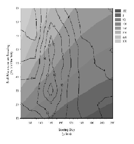
In a recent assessment of the tactical use of seasonal climate forecasts for cropping decisions, Crimp et al. (2007) from CSIRO Sustainable Ecosystems compared six different seasonal climate forecast indices across thirteen different farms in three regions (SE Qld, northern Victoria and WA) with either single decisions or packages of decisions tied to climate forecasts. One of their results for the Victorian site was that even though the benefits of using seasonal forecasts in all years was small, if the forecast was tied to specific soil moisture conditions in a very tight window of opportunity, there could be substantial benefits (Fig 1).

This highlights the benefit of considering other factors such as the level of starting soil water and the break of the season along with the seasonal climate forecast. When seasonal forecasts are considered with other sources of information it becomes clearer that farmers are dealing with evolving information through the season.


Figure 1: Contours of mean gross margin benefit ($/ha, 1957-2006) from using tactically-varied N top-dressing based on the SOI-Phase compared with optimal fixed N top-dressing, for wheat cropping at McClelland’s farm, in the Birchip region. The background shading indicates the baseline gross margins ($/ha) obtained using fixed, ‘optimal’ nitrogen additions.


Looking at a shorter time frame than Seasonal Climate Forecasts – the Madden- Julian Oscillation.

Farmers have often asked about the gap between weather forecasts (4-7 days) and Seasonal Climate Forecasts (3-6 months). Recent research on the Madden-Julian Oscillation (MJO – also known as the 40-day wave) offers some hope here. There is plenty of information on the MJO at http://www.apsru.gov.au/mjo/index.asp that may partly fill this gap. This research shows that the MJO can influence daily rainfall patterns across Australia, especially in the south-east through its influence on synoptic weather systems. This new forecasting capability may be able to improve the tactical management of climate-sensitive systems such as agriculture.

The longer term – climate change
In 2007 it was hard to escape discussion on climate as a source of risk. This was in part due to saturation media coverage to climate change at an international level with the release of the Fourth Assessment Report from the Intergovernmental Panel on Climate Change, but also due to a prolonged drought. In many regions the 2007 cropping season started well and there was a sense that at last a good season was due. This raises questions about whether this event is drought or climate change.

Climate change adds to the uncertainty in using seasonal climate forecasts as it makes the past less useful as a guide to future climate conditions. Furthermore climate change introduces further uncertainty due to the lack of ability to effectively model all the key processes. This is particularly so for longer term projections because of the wide disparity in future climate projections due to alternative assumptions about greenhouse gas emission scenarios as well as the scientific uncertainty. However, somewhat ironically, climate change also may be able to provide us with the most certain thing we can say about the climate several months or a year from now: that it is highly likely to be much warmer than average. The trends in temperature are significant and incessant: Australia has now recorded a warmer-than-average year for 16 of the past 18 years with most of the record warm years occurring within the past two decades. The temperature for 2007 was the sixth warmest on record (0.67°C above average) and 2005 was by far the warmest on record (1.09oC above average). The year 2007 was the warmest year on record for the Murray Darling Basin, South Australia, New South Wales and Victoria. Unfortunately, similar certainty about trends or projections in rainfall currently eludes us.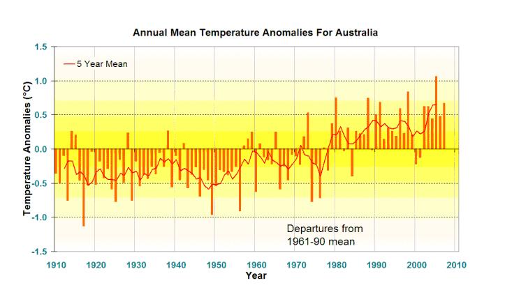 

An excellent source of information on climate change in Australia is the report and interactive website launched in October 2007 by CSIRO and the Bureau of Meteorology http://www.climatechangeinaustralia.gov.au/

Conclusion
Almost one and a half centuries ago in the Times newspaper June 18 1864 the prediction was made “Whatever may be the progress of the sciences, never will observers who are trustworthy and careful of their reputations venture to foretell the state of the weather.”

Perhaps the problem for many grain growers and advisers is that the information from climate science is not good enough to be relied on, but too good to ignore. The challenge is to factor the information, along with all other sources of information into risk management. This is a swing from saying that ‘I heard from this expert or internet site that the season is going to be decile X’, to the less sensational assessment that the probabilities have changed and a wetter season is more likely, but I still need to do my sums on the drier season as there is still some chance that may occurs.


Contact: Peter Hayman
Ph: 08 8303 9729
Email: hayman.peter@saugov.sa.gov.au